|
|
Введение в реверс-инжениринг
Книга представляет из себя вводный курс по reverse engineering
как под Linux , так и под Microsoft Windows.
Мы рассмотрим основные подходы , которые позволяют программисту
раскрывать содержимое черного ящика.
Закрытые проприетарные системы - отличный разражитель для open-source программистов.
Эта книга активно разрабатывается и все еще ищет своего издателя.
Данный текст неполон , в нем много пропусков.
Она не столько о том , как из бинарника получить исходный код ,
сколько о научном дедуктивном методе анализа , выделения и модификации
различной функциональности закрытых программ.
В основном разговор идет на высокоуровневом языке программирования ,
но при необходимости речь переходит на ассемблер.
Книга написана с таким расчетом , чтобы каждый , кто хотя бы прослушал вводный курс по программированию
или на худой конец прочитал Teach Yourself in 21 days,
мог бы в состоянии понять материал.
Знание таких вещей ,как AVL trees, Hash Tables, Graphs, priority queues,
(см.
Design Patterns)
также будет весьма полезным для понимания.
Что такое reverse engineering?
Reverse engineering - технология , позволяющая обходиться без исходников
для того , чтобы модифицировать какой-то софт или понять , как он работает.
Вообще говоря,
reverse engineering - это довольно тяжкий труд ,
и часто требуется команда инженеров , для того чтобы взломать какую-то систему.
Но как бы там ни было , мы узнаем , что есть инструментальные средства ,
которые позволяют найти нужную информацию и хакнуть софт , к которому нет исходников
Ответ : потому что это возможно.
Если у нас есть исходники , у нас есть ключ к пониманию идеологии системы
и возможности управлять ее поведением .
Но так бывает не всегда.
Закрытый софт всегда представляет особый интерес.
Иногда нужно понять , как работает защитная функция,
или взломать защиту .
Это делает вас лучше как программиста
В этой книге есть много чего о том , как работает компьютер на нижнем уровне ,
да и вообще как эффективно писать программы.
To Learn Assembly Language.
Если вы незнакомы с ассемблером , в конце книги есть ссылки . которые помогут вам .
Вы узнаете , как Си генерирует машинный код .
Learn the General Approach
В книге сделан обзор Reverse Engineering
как под UNIX (GNU/Linux) , так и под Microsoft Windows.
Не пытайтесь сфокусировать свое внимание на какой-то одной платформе.
Пытайтесь понять сам процесс выделения информации ,
и как устроены самые различные средства в достижении этой цели.
Use the Scientific Method.
Изучая отдельную программу , вы изучаете систему.
Научный подход можно разбить на несколько шагов :
Выделение и описание какой-то функциональности в программе
Формулировка , обоснование такого поведения
На основе гипотез проникновение внутрь программы и замена кода
Изменение функционала программы вслепую может привести к непредсказуемым результатам.
Большую роль здесь играет последовательность в отладке и тестировании.
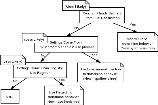
Эта древовидная диаграмма показывает схему отладки под винду,
в конкретных случаях последовательность графов в дереве может значительно отличаться от приведенного.
Например , чтобы узнать , что программа читает из конфигов , можно использовать программу filemon.
Чтобы узнать , как программа инициализирует полученные данные , можно использовать программу procexp.
Чтобы узнать , какая информация берется из регистров , можно узнать с помощью regmon.
![[Tip]](images/reverse/tip.png) | NOTE |
|---|
Если у вас нет стратегии , вы можете потратить большое количество времени на бесполезный обзор
ассемблерного кода.
|
Start with an Aerial View, then Zoom In
Правильный подход заключается в правильной организации шагов .
Но иногда приложение бывает настолько сложным, что непонятно, с чего начать.
В этом случае вам могут помочь : Data Flow
Diagrams и Activity
Diagrams.
Они помогают представить систему в виде нескольких абстрактных уровней.
И вы уже сами можете выбрать нужный уровень.
Data Flow Diagrams моделирует поток данных между исходником, процессом и хранилищем данных.
Chapter 2. The Compilation Process| Revision History |
|---|
| Revision $Revision: 1.4 $ | $Date: 2004/02/12 21:43:34 $ | |
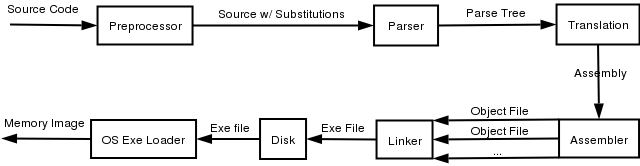
Процесс компиляции можно разбить на 5 стадий : Preprocessing,
Parsing, Translation, Assembling, Linking.
В данной схеме мы рассматриваем юниксовый компилятор - gcc
(или g++). Последовательность такова :
gcc -> gcc -E -> gcc -S -> as -> ld.
Под виндой процесс несколько более другой , но в рамках MSVC++ в принципе все то же самое.
Под винду также есть версия гну-шного компилятора,
смотрите MinGW project или
Cygwin
Project.
Cygwin генерит POSIX-совместимый код .
MinGW позволяет строить нативные виндовые приложения.
Генерация бинарного исполняемого файла выполняется компилятором.
Это справедливо и для юникса , и для винды.
gcc - C-ный компилятор для UNIX.
Для вывода протокола пошаговых действий , выполняемых gcc , нужно набрать опцию gcc -v
cl.exe выполняет аналогичную функцию в случае с MSVC++ под виндой.
Попробуйте набрать cl -? .
Если вы запускаете cl.exe не из среды MSVC++ ,
нужно позаботиться о путях и системных переменных компиляции
- в этом вам поможет системный батник vsvars32.bat ,
который обычно можно найти в подкаталоге CommonX/Tools.
Препроцессор - это все , что стоит после # и управляет логикой компиляции на С .
gcc -E
выполняет лишь одну стадию препроцесса.
Будут подключены хидеры и макросы переведены в нормальный код.
Добавление опции -o file укажет редирект на обьектный файл.
Parsing And Translation Stages
Парсинг и трансляция - наиболее полезные для нас стадии компиляции.
Юниксовый и виндовый синтаксисы ассемблеров , к сожалению , различаются.
Юниксовый ассемблер в свою очередь , как известно , имеет интеловский диалект ,
а также AT-шный. Переключение между ними не должно составлять большого труда.
Опция gcc -S
генерит из .c файлов ассемблерные файлы .s с синтаксисом
AT&T.
Если вы хотите получить интеловский синтаксис , добавьте опцию
-masm=intel. Для генерации переменных стека
используйте опцию -fverbose-asm.
gcc имеет опцию оптимизации.
Можно задать опцию оптимизации -ON, где 0 <= N <= 6.
0 - нет оптимизации , 6 - максимальная оптимизация.
Есть также несколько опций , задаваемых с помощью флага -f.
Некоторые из них: -funroll-loops, -finline-functions, -fomit-frame-pointer.
Loop unrolling - создаются n копий для n итераций цикла и полностью отсутствуют директивы jmp.
На новейших процах эта опция практически не дает эффекта.
Инлайн-опция означает конвертацию функций в макросы.
Omit-опция освобождает регистры для их эффективного использования,
что дает выигрыш при большом количестве локальных переменных.
| NOTE |
|---|
У всех этих опций есть соответствующие анти-опции : например опция -fno-inline-functions
имеет обратное действие для опции -finline-functions.
С помощью опции -fverbose-asm опции компиляции будут распечатаны
в заголовке ассемблерного файла.
Недостатком gcc-3.x является то . что он все равно делает оптимизацию , даже если мы включили опцию
уровня -O0.
Отключение оптимизации делается с помощью опции -fno-.
|
Аналогично , cl.exe имеет опцию -S для генерации ассемблера,а также опции оптимизации.
К сожалению , cl не позволяет это делать в той же степени , что и gcc.
Похожие опции для cl.exe :
-Ob<n> - inline functions (-finline-functions)
-Oy - enable frame pointer omission (-fomit-frame-pointer)
Это стадия перевода ассемблерного кода в машинные инструкции.
Тут могут происходить небольшие сюрпризы , такие , как смена порядка команд.
as - GNU-шный assembler.
Он может компилировать как синтаксис AT&T , так и Intel syntax,
генерируя при этом обьектные файлы .o
MASM - Microsoft assembler.
Винда и юникс имеют схожие линковочные процедуры.
Обе системы поддерживают 3 стиля линковки.
- Static Linking
В этом случае код всех функций находится внутри самого исполняемого файла.
- Dynamic Linking
При динамической линковке где-то отдельно лежит библиотека функций ,
и ее виртуальное пространство будет прикручено операционной системой
к адресному пространству исполняемого файла.
Вызовы таких библиотечных функций будут сгенерированы в момент компиляции программы
и помещены в Procedure Linkage Table, или PLT.
- Runtime Linking
Runtime-линковка происходит на лету , в момент выполнения уже откомпилированной программы.
В юниксе для этого используется системный вызов dlopen(),
под виндой это LoadLibrary().
ld - GNU-шный линкер.
Он непосредственно генерит исполняемый файл.
Это MSVC++ linker. Для его вызова нужно задать опцию cl -link .
Для генерации .dll вы должны иметь предварительно соответсвующие библиотеки .lib (или .def).
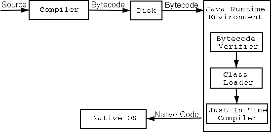
Java , как известно , интерпертатор , и отличается от C/C++.
Программы тут выполняются на т.н. Java Virtual Machine ( JVM),
и реализовано это с помощью интерпретатора.
Java-код не компилируется в исполняемый код ,
вместо этого происходит компиляция т.н. промежуточного байт-кода,
который и выполняется на виртуальной маштне.
Java-класс размещается в отдельном исходном файле, имеющем имя самого класса и расширение
.java.
При компиляции каждый класс оказывается размещенным в собственном бинарном
.class-файле.
2 уникальные фазы - class loader и bytecode verifier - отличаю Java от C/C++.
class loader загружает class' bytecode.
Разработчик может написать свой собственный class loader.
При загрузке класса виртуальной машиной вызывается метод loadClass(String name, boolean resolve);.
Далее класс передается в память через метод defineClass.
Если класс не найден , может быть загружен родительский класс либо вызван метод
findSystemClass.
Природа Lava-bytecode позволяет сравнительно легко декомпилировать байткод в исходник.
Chapter 3. Gathering Info| Revision History |
|---|
| Revision $Revision: 1.4 $ | $Date: 2004/01/31 20:56:53 $ | |
Первый шаг для понимания программы - получение информации о ней с помошью других программ.
System Wide Process Information
Как в винде , так и в линуксе есть приложения , которые дают информацию
о выполняющихся процессах.
Файловая линуксовая система /proc вмещает в себя различную информацию ,
начиная от зависимых библиотек и кончая сокетами.
/proc имеет каталог для каждого выполняемого процесса.
Если у процесса pid=1337, то соответсвенно имеется каталог /proc/1337/.
Вы можете наблюдать только те процессы , которые запустили именно вы.
Интересные параметры в этом каталоге :
cmdline -- список командных параметров процесса
cwd -- линк на рабочую директорию процесса
environ -- список переменных окружения процесса
exe -- линк на выполняемый файл
fd -- список файловых дескрипторов , используемых процессом
maps -- список memory locations процесса,
которые можно напрямую посмотреть с помощью gdb/
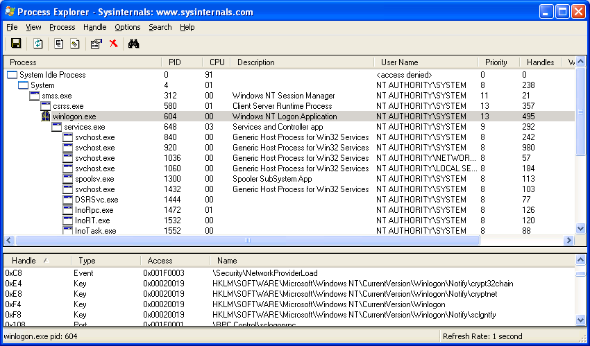
Sysinternals Process Explorer
Sysinternals
- эта известная марка предоставляет набор утилит под винду.
Process Explorer показывает зависимые dll-ки,
функции и соответсвующие им адреса , security attributes, открытые файлы,
тип управляемых обьектов и т.д. Эта утилита позволяет модифицировать процесс.
Можно управлять хэндлами , пермишинами , дебажить и т.д.
Obtaining Linking information
Для понимания работы программы нужно собрать информацию об используемых библиотеках.
Юниксовый ldd - это основная утилита для сбора информации о прилинкованных библиотеках.
Она дает информацию о маппированных адресах внутри адресного пространства программы.
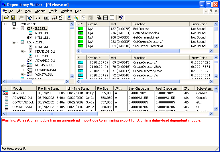
depends - утилита , идущая в поставке Microsoft
SDK,
либо MS Visual Studio.
Она показывает не только список dll-ек , но и функции внутри них,
характер их импорта.
Когда вы кликаете на dll-ке , вы получаете список импортируемых функций (зеленая окраска).
Вы также получаете список экспортируемых функций.
Используемые покрашены в синий цвет , неиспользуемые - в серый.
Иногда функция может быть "bound", в этом случае ее модификация затруднительна.
Obtaining Function Information
Следующий шаг - идентификация функциональных блоков программы.
Юниксовый nm выводит список функций , глобальных переменных , и их адреса внутри бинарника.
В винде есть аналог - dumpbin.exe,возможности которого поменьше.
Он выводит список импортируемых/экспортируемых функций.
К тому же эти функции должны иметь префикс __declspec( dllexport )
Viewing Filesystem Activity
Юниксовый lsof показывает список всех открытых файлов , используемых процессом.
Это может быть обычный файл , каталог, block file, character special file,
ссылка, библиотека, поток или сетевой файл(Internet socket, NFS file или UNIX domain socket).
lsof как правило не инсталлируется по умолчанию на систему.
В некоторых дистрибутивах он лежит в /usr/sbin.
Пример вывода: COMMAND PID USER FD TYPE DEVICE SIZE NODE NAME
bash 101 nasko cwd DIR 3,2 4096 1172699 /home/nasko
bash 101 nasko rtd DIR 3,2 4096 2 /
bash 101 nasko txt REG 3,2 518140 1204132 /bin/bash
bash 101 nasko mem REG 3,2 432647 748736 /lib/ld-2.2.3.so
bash 101 nasko mem REG 3,2 14831 1399832 /lib/libtermcap.so.2.0.8
bash 101 nasko mem REG 3,2 72701 748743 /lib/libdl-2.2.3.so
bash 101 nasko mem REG 3,2 4783716 748741 /lib/libc-2.2.3.so
bash 101 nasko mem REG 3,2 249120 748742 /lib/libnss_compat-2.2.3.so
bash 101 nasko mem REG 3,2 357644 748746 /lib/libnsl-2.2.3.so
bash 101 nasko 0u CHR 4,5 260596 /dev/tty5
bash 101 nasko 1u CHR 4,5 260596 /dev/tty5
bash 101 nasko 2u CHR 4,5 260596 /dev/tty5
bash 101 nasko 255u CHR 4,5 260596 /dev/tty5
screen 379 nasko cwd DIR 3,2 4096 1172699 /home/nasko
screen 379 nasko rtd DIR 3,2 4096 2 /
screen 379 nasko txt REG 3,2 250336 358394 /usr/bin/screen-3.9.9
screen 379 nasko mem REG 3,2 432647 748736 /lib/ld-2.2.3.so
screen 379 nasko mem REG 3,2 357644 748746 /lib/libnsl-2.2.3.so
screen 379 nasko 0r CHR 1,3 260468 /dev/null
screen 379 nasko 1w CHR 1,3 260468 /dev/null
screen 379 nasko 2w CHR 1,3 260468 /dev/null
screen 379 nasko 3r FIFO 3,2 1334324 /home/nasko/.screen/379.pts-6.slack
startx 729 nasko cwd DIR 3,2 4096 1172699 /home/nasko
startx 729 nasko rtd DIR 3,2 4096 2 /
startx 729 nasko txt REG 3,2 518140 1204132 /bin/bash
ksmserver 794 nasko 3u unix 0xc8d36580 346900 socket
ksmserver 794 nasko 4r FIFO 0,6 346902 pipe
ksmserver 794 nasko 5w FIFO 0,6 346902 pipe
ksmserver 794 nasko 6u unix 0xd4c83200 346903 socket
ksmserver 794 nasko 7u unix 0xd4c83540 346905 /tmp/.ICE-unix/794
mozilla-b 5594 nasko 144u sock 0,0 639105 can't identify protocol
mozilla-b 5594 nasko 146u unix 0xd18ec3e0 639134 socket
mozilla-b 5594 nasko 147u sock 0,0 639135 can't identify protocol
mozilla-b 5594 nasko 150u unix 0xd18ed420 639151 socket
Краткий комментарий вывода :
   cwd  current working directory
     mem  memory-mapped file
     pd   parent directory
     rtd  root directory
     txt  program text (code and data)
     CHR  for a character special file
     sock for a socket of unknown domain
     unix for a UNIX domain socket
     DIR  for a directory
     FIFO for a FIFO special file
| fuser |
|---|
Схожий функционал имеет утилита fuser. У нее в качестве параметра можно задать имя файла или сокета
и получить pid процесса , который имеет доступ к этому файлу.
|
Аналогом lsof в винде является утилита Sysinternals Filemon.
Она показывает открытые файлы , а также запросы на чтение/запись.
Реестр в винде - ключ к понимаю системы , он хранит в себе массу секретов.
Regmon мониторит все активно используемые разделы реестра.
Viewing Open Network Connections
В данном случае имя утилиты совпадает и для винды , и для юникса -
речь идет о netstat.
Эта утилита есть чуть ли ни во всех операционных системах.
ее можно использовать для мониторинга сетевых коннектов , роутинг-таблиц и т.д.
Если исследуемая программа использует сетевую коммуникацию,
мы можем определить внешние хосты , куда идет коннект,
причем речь идет не только о TCP.
Пример вывода :
| NOTE |
|---|
Показан юниксовый вывод . Под винду почти все то же самое.
|
В данном случае вывод разделен на 2 части -
Internet connections и UNIX domain sockets.
Первый столбец - имя протокола.
Следующие два - получаемые и отсылаемые пакеты.
Затем - source host/port, destination host/port.
Последний столбец - состояние коннекта.
В TCP-коннекте присутствует несколько стадий - ESTABLISHED . SYN_SENT, TIME_WAIT, LISTEN.
В зависимости от опций netstat на экран можно выводить еще больше информации.
Опция -a показывает все коннекты .
Опция -n показывает IP-адреса в числовом виде.
 netstat -p as normal user
 (Not all processes could be identified, non-owned process info
  will not be shown, you would have to be root to see it all.)
 Active Internet connections (w/o servers)
 Proto Recv-Q Send-Q Local Address           Foreign Address         State       PID/Program name
 tcp        0      0 slack.localnet:58705    egon:ssh                ESTABLISHED -
 tcp        0      0 slack.localnet:58766    winston:www             ESTABLISHED 5587/mozilla-bin
 netstat -npa as root user
 Active Internet connections (servers and established)
 Proto Recv-Q Send-Q Local Address           Foreign Address         State       PID/Program name
 tcp        0      0 0.0.0.0:139             0.0.0.0:*               LISTEN      390/smbd
 tcp        0      0 0.0.0.0:6000            0.0.0.0:*               LISTEN      737/X
 tcp        0      0 0.0.0.0:22              0.0.0.0:*               LISTEN      78/sshd
 tcp        0      0 10.0.0.3:58705          128.174.252.100:22      ESTABLISHED 13761/ssh
 tcp        0      0 10.0.0.3:51766          10.0.0.1:22             ESTABLISHED 897/ssh
 tcp        0      0 10.0.0.3:51765          10.0.0.1:22             ESTABLISHED 896/ssh
 tcp        0      0 10.0.0.3:38980          128.174.252.105:22      ESTABLISHED 8272/ssh
 tcp        0      0 10.0.0.3:58510          128.174.5.39:22         ESTABLISHED 13716/ssh
Данный вывод показывает , что мозилла устанавливает коннект с winston ( port - www(80)).
SMB daemon, X server, и ssh daemon стоят на прослушивании.
Сбор сетевой информации обычно выполняется с помощью сниферов.
ethernet card устанавливается в режим promiscuous mode и анализируется весь траффик , проходящий через нее.
Что такое promiscuous mode?
Ethernet - это broadcast media, или устройство , которой является промежуточным звеном
в передаче сетевого трафика.
Каждый сетевой интерфейс (network interface card -NIC)
имеет свой уникальный идентификатор - MAC (Media Access Control).
Все пакеты , идущие по локальной сети , в режиме promiscuous mode
могут читаться сетевым интерфейсом , независимо от того , какой у этих пакетов пункт назначения.
|
Есть несколько наиболее популярных снифферов , с различным интерфейсом и возможностями.
Вот они :
ethereal -
один из лучших снифферов.
Имеет графический GTK-интерфейс. Кроме того что он сниффер , он еще и протокольный анализатор.
Он анализирует в том смысле , что например для TCP-протокола он может показать
флаги SYN , ACK, или kerberos или NTLM -хидеры.
Есть версия как под винду , так и под линукс.
Для него требуется библиотека pcap. Доступен www.ethereal.com
, также вам понадобится
libpcap для Linux или WinPcap для Microsoft Windows.
tcpdump -
один из первых снифферов. Это консольное приложение.
Он встроен в большинство линуксовых дистрибутивов.
Версия для Microsoft Windows - WinDump.
ettercap -
еще один консольный сниффер.
Использует ncurses-библиотеку для консольного GUI.
Он построен на основе ARP.
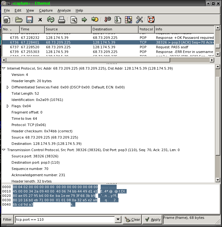
Рассмотрим задачу : как происходит аутентификация mail-клиента и как он забирает сообщения с сервера.
Протокол - POP3, и мы говорим снифферу ethereal забирать трафик с порта 110.
Для входящего и исходящего трафика установим опцию
tcp.port == 110.
Пример сеанса работы ethereal:
Ethereal разбивает пакеты, показывая версию Internet Protocol 4.
Chapter 4. Determining Program Behavior
| Revision History |
|---|
| Revision $Revision: 1.3 $ | $Date: 2004/01/31 20:56:53 $ | |
There are a couple of tools that allow us to look into program
behavior at a more closer level. Lets look at some of these:
This section is really only relevant for to our efforts under UNIX, as
Microsoft Windows system calls change regularly from version to version, and have
unpredictable entry points.
These programs trace system calls a program makes as it makes them.
Useful options:
-f (follow fork) -ffo filename (output trace to filename.pid for
forking) -i (Print instruction pointer for each system
call)
Now we're starting to get to the more interesting stuff. Tracing library
calls is a very powerful method of system analysis. It can give us a
*lot* of information about our target.
This utility is extremely useful. It traces ALL library calls made by a
program.
Useful options:
-S (display syscalls too) -f (follow fork) -o filename (output trace to filename) -C (demangle C++ function call names) -n 2 (indent each nested call 2 spaces) -i (prints instruction pointer of caller) -p pid (attaches to specified pid)
API
Monitor is incredible. It will let you watch .dll calls in real
time, filter on type of dll call, view
Chapter 5. Determining Interesting Functions| Revision History |
|---|
| Revision $Revision: 1.2 $ | $Date: 2004/01/25 16:57:43 $ | |
Clearly without source code, we can't possibly hope to understand all
of sections of an entire program. So we have to use various methods and
guess work to narrow down our search to a couple of key functions.
Reconstructing function & control information
The problem is that first, we must determine what portions of the code
are actually functions. This can be difficult without debugging symbols.
Fortunately, there are a couple of utilities that make our lives easier.
Objdump's most useful purpose is to disassemble a program with the -d
switch. Lacking symbols, this output is a bit more cryptic. The -j option
is used to specify a segment to disassemble. Most likely we will want
.text, which is where all the program code lies.
Note that the leftmost column of objdump contains a hex number. This
is in fact the actual address in memory where that
instruction is located. Its binary value is given in the next column, followed by
its mnemonic.
objdump -T will give us a listing of all library functions this program
calls.
Steve Barker wrote a neat little
perl script that makes objdump much more legible in the
event that symbols are not included. The script has since been extended and
improved by myself and Nasko Oskov. It now makes 3 passes through the output.
The first pass builds a symbol table of called and jumped-to locations.
The second pass finds areas between two rets, and inserts them into the symbol
table as "unused" functions. The third pass prints out the nicely labeled
output, and prints out a function call tree. Usage:
./disasm /path/to/binary > binary.asminfo There are/will be few command line options to the utility. Now
--graph is supported. It will generate a file called call_graph that
contains definition that can be used with a program called dot to
generate visual representation of the call graph.
Note: Unused functions just mean that that function wasn't called
DIRECTLY. It is still possible that a function was called through a
function pointer (ie, main is called this way)
Ok, so now we're getting ready to get really down and dirty. The first
step to finding what you are looking for is to know what you are
looking for. Which functions are 'interesting' is entirely dependent on your point
of view. Are you looking for copy protection? How do you suspect it is
done. When in the program execution does it show up? Are you looking
to do a security audit of the program? Is there any sloppy string usage?
Which functions use strcmp, sprintf, etc? Which use malloc? Is there a
possibility of improper memory allocation?
If we can narrow down our search to just a few functions that are
relevant to our objective, our lives should be much easier.
Regardless of our objective, it is almost always helpful to know where
main() lies. Unfortunately, when debugging symbols are removed, this is
not always easy.
In Linux, program execution actually begins at the location defined by
the _start symbol, which is provided by gcc in the crt0 libraries (check
gcc -v for location). Execution then continues to __libc_start_main(),
which calls _init() for each library in the program space. Each _init() then
calls any global constructors you may
have in that particular library. Global constructors can be created by
making global instances of C++
classes with a constructor, or by specifying
__attribute__((constructor)) after a function prototype. After this,
execution is finally transferred to main through an indirect call
off of the base register ebp.
The easiest technique is to try to use our friends ltrace and gdb
(FIXME: the debugging chapter has been moved to after this one..)
together with our disassembled output. Checking the return address of
the first few functions of ltrace -i, and cross referencing that to our
assembly output and function call tree should give us a pretty good idea
where main is. We may have to try to trick the program into exiting
early, or printout out an error message before it gets too deep into its
call stack.
Other techniques exist. For example, we can LD_PRELOAD a .c file with a
constructor function in it. We can then set a breakpoint to a libc
function that it calls that is also in the main executable, and
finish and stepi
until we are satisfied that we have found main.
Even better, we could just set a breakpoint in the function
__libc_start_main (which is a libc function, and thus we will always
have a symbol for it), and do the same technique of finishing and
stepping until we reach what looks like main to us.
At worst, even without a frame pointer, we should be able to get the
address of a function early enough in the execution chain for us to
consider it to be main.
Finding other interesting functions
Its probably a good idea to make a list of all functions that call exit.
These may be of use to us.
Other techniques for tracking down interesting functions include:
Checking for which functions call obscure gui construction
widgets used in a dialog box asking for a product serial number
Checking the string references to find out which
functions reference strings that we are interested in. For
example, if a program outputs the text "Already registered."
knowing what function outputs this string is helpful in figuring
out the protection this particular program uses.
Running a program in gdb, then hitting control C when it begins
to perform some interesting operation. using stepi N should slow things
down and allow you to be more accurate. Sometimes this is too slow
however. Find a commonly called function, set a breakpoint, and try
doing cont N.
Checking which functions call functions in the BSD socket layer
Plotting out program flow
Plot out execution paths into a tree from main, especially to your
function(s) of interest. You can use disasm.pl to generate call graphs
with the --graph option. Using it enables the script to generate file
called call_graph. It contains definition of the call graph in a
format used by a popular graphing tool called dot. Feeding this
definition file in dot will give you a nice (probably pretty huge)
graphics file with visual representation of the call graph. It is
pretty amazing. Definitely try it with some small program.
Further analysis will have to hold off until we understand some assembly.
Chapter 6. Understanding Assembly| Revision History |
|---|
| Revision $Revision: 1.3 $ | $Date: 2004/02/25 21:04:10 $ | |
Since the output of all of these tools is in AT&T syntax, those of you
who know Intel/MASM syntax have a bit of
re-learning to
do.
Assembly language is one step closer to the hardware than high level
languages like C and C++. So to understand assembly, you have to
understand how the hardware works. Lets start with a set of memory
locations known as the CPU registers.
Registers are like the local variables of the CPU, except there are a
fixed number of them. For the ix86 CPU, there are only 4 main registers
for doing integer calculations: A, B, C, and D. Each of these 4
registers can be accessed 4 different ways: as a 32 bit value (%eax),
as a 16 bit value (%ax), and as a low and a high 8 bit value
(%al and %ah). There are five more registers that you will see used
occasionally - namely SI, DI, SP and BP. SI and DI are around
from the DOS days when people used 64k segmented addressing, and as it
turns out, may be used as integer like normal registers now. SP and BP
are two special registers used to handle an area of memory called the
stack. There is one last register, the instruction pointer IP that you
may not modify directly, but is changed through jmps and calls. Its
value is the address of the next instruction to execute.
(FIXME: Check this)
Note: If gcc was called with the -fomit-frame-pointer, the BP register
is freed up to be used as an extra integer register.
A stack is what is called a Last In, First
Out data structure or LIFO. Think of it as a stack of plates. The most
recent (last) plate pushed on top of the stack is the first one to be
removed. This allows us to manage the stack with only one register if
need be, namely the stack pointer or SP register.
The stack is a region of memory that is present throughout the entire
lifetime of a program. It is where local variables are stored, and it is
also how function call arguments are passed.
On almost all modern computers, the stack is said to grow down, that is, as
elements are pushed on to it, the SP register is decremented by the size
of the element pushed. From our earlier analogy, its as if the stack of
plates where hung from the ceiling, new plates were inserted at the
bottom, and the whole stack some sort of catch to stop
them all from dumping out. That catch would be the SP register.
So the stack starts from a high memory address,
and works down to a lower address. This is because another section of
memory called the heap grows up, and its handy to have the two of them
grow towards eachother to fill in a single empty hole in the program
address space.
Note: It is easy to become confused when dealing with the
stack. Remember that while it may grow down, variables are still
addressed sequentially upwards. So an array of char b[4] at esp of 80
will have b[0] at 80 (right at the stack pointer), b[1] above that at
81, b[2] at 82, and b[3] at 83, which is where the stack pointer was
before the push. The next push will then place the stack pointer at 76.
There are two instructions that deal with the stack directly: push and
pop. Each take a register or value as an argument. Push will place its
argument onto the stack, and then decrement the SP by the size of its
argument (4 for pushl, 2 for pushw, 1 for pushb).
//FIXME (What is pushl and push b)
Pop copies the value on the top of
the stack into its argument, then increments SP.
Pusha and popa push and pop all the registers with one instruction.
Because of speed
considerations, the value is not touched, just the SP register is
changed to point to the next location ot the stack. So SP is always
pointing to the top value of the stack and not at invalid memory.
Normal arithmetic expressions can also be used to modify SP to make
space for working directly with stack memory with other instructions.
How gcc works with the stack
Right before a function is called, its arguments are pushed onto the stack in
reverse order. Then the call instruction pushes the address of the next
instruction (ie the value of IP after call) onto
the stack, and then the CPU begins executing
the address of the call by copying that value into the invisible
instruction pointer (IP) register.
The called function then starts with what is known as the function
prolog, which pushes the current base pointer onto the stack, and then
copies the current stack pointer to the base pointer, and then subtracts
from SP enough space to hold all local variables (and then some!).
The base pointer is then used to reference variables and parameters during
function execution, since its value is not affected by pushes and pops. Thus,
parameters all have fixed positive offsets from the BP, where as local
variables all have fixed negative offsets from the BP.
At the end of function execution, the base pointer is copied to the stack
pointer during ret, and the return address is popped off the stack and
placed into the invisible IP register to return to the caller function.
Note: Unless -fomit-frame-pointer is specified, gcc always generates code that
references local variables by negative offsets from the BP instead of
positive offsets from the SP.
Two's complement is specific way signed integers are represented in pretty
much all modern computers. This is due to the fact that two's complement
form has several advantages:
The same rules for addition apply, no extra work is required to
compute the sum of negative integers. Easy to negate a number. The most significant bit tells you the sign: 0 is positive, 1
is negative.
It should be noted that when using signed values the ranges of number
that can be represented by a specific number of bits is less than the
usual. The range is -(2n-1) to
+(2n-1)-1
There are several ways to convert any unsigned binary number into signed
two's complement form.
The most intuitive and easy to remember is the following
Complement each bit of the number and add one. Let's find how -13 is
represented, so we convert it into its binary form:
0000 1101

 Then invert all the bits.
 1111 0010

 Now add one to it.
 1111 0011

 So 1111 0011 is -13 in two's complement.
Second method is to complement all the bits to the left of the rightmost
1 bit, but not including it (but not the rightmost bit, for example 0001
0100). It sounds a bit complicated, but is easier
once you figure out how it is done. Let's get back to the example of -13.
0000 1101
         ^
 Invert the bits to the left of the rightmost one.
 1111 0011
There you go. We get the number without second step of adding one. It can
be proven why this method works, but we are not in class.
Yet a third method is to subtract the number from
2n. Here is how it works.
 1000 0000
 -
  0000 1101
  ---------
  1111 0011
There may be other ways of doing it, but if you master those, you will
not need to remember any more.
To convert a negative number in two's complement, you apply the exact
same procedure as described and you get back the positive value for the
number.
From reverse engineering angle
Now that we know what two's complement is let's look at some examples of
this type of representation in reverse engineering process. Using one of
the tools discussed earlier, objdump and the wrapper disasm.pl, let's
look at the ls command binary. If you look at function7 (which starts at
address 80495a8), lines like the following appear frequently:
80495be: 83 c4 f8 add $0xfffffff8,%esp
What does this instruction do? It just adds some constant to the stack
pointer register (%esp). There are two ways you can look at this
constant. It is either a huge unsigned number or two's complement
negative number. Since we just add to the stack pointer, it does not
make sense to be big number, so let's find what is the value of this
number.
  f    f    f    f    f    f    f    8
 1111 1111 1111 1111 1111 1111 1111 1000

 0000 0000 0000 0000 0000 0000 0000 1000
   0    0    0    0    0    0    0    8
Now we can see that this is just the negative of 0x00000008 or just
plain -8 in decimal. If you think about this, what this line does is
decrement the stack pointer by 8 bytes (allocate more space).
One common difficulty in working on multiple platforms is that different
platforms use different byte orders.
Byte ordering refers to the physical layout of integer data in memory.
There are two different orderings - little endian and big
endian.
When a
data structure or data type is represented by more than one byte, the
ordering of bytes matters. For example if we consider a long (4 bytes) let's label
the least significant byte 0 and the most significant one 3. If we are on little
endian machine the long will be represented in memory like this (yeah, some
machines do not allow addressable bytes, but let's forget about this):
     0x040   0
      0x041   1
      0x042   2
      0x043   3
On a big endian machine on the other hand, the long will be layed out
like that:
     0x040   3
      0x041   2
      0x042   1
      0x043   0
Now let's look at an example. The easiest way to see the difference in
byte ordering is to look at how a long is stored in memory on different
architectures. Here is an example program that will demonstrate it.
#include <stdio.h>

 int main() {

     long longval = 123456789;

     printf("%s\n", test);

 }
After compiling it with debugging info, let's run it and see what will
be the result. The first run is on Intel-based machine.
bash$ uname -a
 Linux slack 2.4.20 #5 Tue Dec 31 00:01:00 CST 2002 i686 unknown
bash$ gdb ./a.out
 GNU gdb 5.2.1
 This GDB was configured as "i386-slackware-linux"...
 (gdb) break main
 Breakpoint 1 at 0x8048338: file test.c, line 5.
 (gdb) run
 Breakpoint 1, main () at test.c:5
 5               long longval = 123456789;
 (gdb) stepi
 8               printf("value is %d\n", longval);

 Let's get the address of longval in memory
 (gdb) print &longval
 $2 = (long int *) 0xbffff234

 Let's print the contents of longval as a word
 (gdb) x/w 0xbffff234
 0xbffff234:     0x075bcd15

 Let's print the contents of longval as 4 consecutive bytes
 (gdb) x/4b 0xbffff234
 0xbffff234:     0x15    0xcd    0x5b    0x07
 (gdb) quit
The second run was on Sparc machine running Solaris.
remsun1> uname -a
 SunOS remsun1 5.8 Generic_108528-16 sun4u sparc SUNW,Sun-Fire-280R
remsun1> gdb ./a.out
 GNU gdb 4.18
 This GDB was configured as "sparc-sun-solaris2.7"...
 (gdb) break main
 Breakpoint 1 at 0x10564: file test.c, line 5.
 (gdb) run
 Breakpoint 1, main () at test.c:5
 5               long longval = 123456789;
 (gdb) stepi
 0x10568 5               long longval = 123456789;

 Let's get the address of longval in memory
 (gdb) print &longval
 $1 = (long int *) 0xffbefaec

 Let's print the contents of longval as a word
 (gdb) x/1w 0xffbefaec
 0xffbefaec:     0x075bcd15

 Let's print the contents of longval as 4 consecutive bytes
 (gdb) x/4b 0xffbefaec
 0xffbefaec:     0x07    0x5b    0xcd    0x15
 (gdb)
One can clearly see how on the Sparc machine the individual bytes are in
the same order as in the printed word, whereas the Intel machine has it
reverse.
This is the difference in byte ordering. In order for different hosts on
the same network to be able to communicate and the exchanged data to make
sense, they agree on common byte ordering. In modern networking the data is
transmitted in big endian byte ordering i.e. most significant byte comes
first. On the i80x86 the host byte order is Least Significant Byte first,
whereas the network byte order, as used on the Internet, is Most Significant Byte
first.
Keep track of the stack and registers
The secret to understanding assembly code is to always work with a
sheet of paper and a pencil. When you first sit down, draw out a table
for all 6 registers A, B, C, D, SI, and DI. Keep track of the high
and low portions as well. Each new line of this table should represent a
modification of a register, so the last value in each register column is
the current value of that register.
Next, draw out a long column for the stack, and leave space on the sides
to place the BP and SP registers as they move down. Be sure to write all
values into the stack as they are placed there, including ret and the
stored BP.
In AT&T syntax, all instructions are of the form:
mnemonic src, dest
Standalone numerical constants are prepended with a $. Hexadecimal
numbers always start with 0x (as opposed to ending in h). Registers are
specified with a % sign, ie %eax.
Dereferencing or pointer representation is of the form
disp(%base, %index, scale), where the resulting address is
disp + %base + %index*scale. disp and scale are constants (no $), and
%base and %index are registers. Any of these 4 may be omitted, leaving
either blank space and then a comma, or simply leaving off the argument, and all
remaining arguments. For example, 4(%eax) means memory address 4+%eax,
where as (,%eax,4) means %eax*4. This compact notation makes array
indexing easy.
From here, it is simply a matter of understanding what each assembly
mnemonic does. Most common mnemonics are obvious, but you can
find a complete description of all the Intel instructions (in agonizing
detail) at
Intel's
Developer Site. Volume 2 contains the instruction list. Keep in
mind that in Intel syntax, operands are in the reverse order of
AT&T syntax (ie, mnemonic dest,src).
In order to learn to read assembly effectively, you really have to know
what type of code your compiler likes to generate in certain situations.
If you learn to recognize what a while loop, a for loop, an if-else
statement all look like in assembly, you can learn to get a general feel
for code more quickly. There are also a few tricks that GCC performs that
may seem unintuitive at first to the neophyte reverse engineer, even if
they already know how to forward-engineer in assembly.
In assembly, the only flow control mechanisms are branching and
calling. So every control structure is built up from a combination of
goto's and conditional branches. Lets look at some specific examples.
So we've mentioned that function calls use the stack to pass arguments.
But where does that leave return values? And what about local variables?
Local variables are also on the stack, just below the base pointer
instead of above. But if you thought that a return value was a pop off of the
stack, you were wrong! GCC places the return value of a particular function
into the eax register at the end
of that function. Upon calling a function with a return value, it knows
to copy the eax register into whatever variable will store that return
value.
So lets see some gcc output for function calls. Get your paper
ready, we're going to need to draw our stack and register table to
follow these. Yeah yeah, it seems like a hassle, and you're sure you
can do without it. We know, we know. But humor us. If you at least
practice the methodical way a few times, doing things in your head
will become easier later.
gcc 2.95
Example .c file
and gcc output with
no optimization, with
-O2, and with
-O3
-fomit-frame-pointer To get the most out of these examples,
start at main, and trace execution throughout the executable. Do the
low optimization first, and then move up to higher levels. The
comments assume you are progressing in that order. FIXME: We may want
to split these out into several simpler example files, to avoid
overwhelming people all at once.
gcc 3.3.2
The same files are also compiled with gcc version 3.3.2 and the
corresponding files are
functions.c,
no
optimization,
-O3
-fomit-frame-pointer.
The if statement is represented in assembly as a test followed by a
jump. The thing to notice is that sometimes the body of the if
statement is what is jumped to, as opposed to being jumped over as your
C code may specify. This means that the condition for the jump will
often be the negation of the condition for your if statement.
gcc 2.95
Example .c file and gcc output
with no optimization, with
-O2, and with
-O3 -fomit-frame-pointer
gcc 3.3.2
The same files are also compiled with gcc version 3.3.2 and the
corresponding files are
if.c,
no optimization,
-O3
-fomit-frame-pointer.
Complicated if statements
Of course, if statements can get much more complicated than the above
examples. They can contain boolean short-circuits, function calls,
nested-ifs, etc.
Arrays on the stack are just memory regions that we access with
variations on the disp(%base, %index, scale) idea presented earlier. So lets
start with a warm-up consisting of a simple char array where we let libc do
all the work.
gcc 2.95
Example .c file and gcc output
with no optimization, with
-O2, and with
-O3 -fomit-frame-pointer
gcc 3.3.2
array-stack-char.c,
no optimization,
-O3 -fomit-frame-pointer
So lets do another example where we do all the work. One dimensional
arrays are the easiest, as they are simply a chunk of memory that
is the number of elements times the size of each element.
gcc 2.95
Example .c file and gcc output
with no optimization, with
-O2, and with
-O3 -fomit-frame-pointer
gcc 3.3.2
array-stack-int1D.c,
no optimization,
-O3 -fomit-frame-pointer
Two dimensional arrays are actually just an abstraction that makes
working with memory easier in C. A 2D array on the stack is just one long 1D
array that the C compiler divides for us to make it manageable. To parameterize
things, an array declared as: type array[dim2][dim1]; is really a 1D array of
length dim2*dim1*type. The C compiler handles array indexing as follows:
array[i][j] is the memory location array + i*dim1*type + j*type. So it divides
our 1D array into dim2 sections, each dim1*type long.
FIXME: Graphics to illustrate this.
gcc 2.95
Example .c file and gcc output
with no optimization, with
-O2, and with
-O3 -fomit-frame-pointer
gcc 3.3.2
array-stack-int2D.c,
no optimization,
-O3 -fomit-frame-pointer
As I tell my introductory computer science students, the best way to
think of higher dimensional arrays is to think of a set of arrays of the next
lower dimension. So the best way to think about how a 3D array can be jammed
into a 1D array is to think about how a set of 2D arrays would be jammed into
a 1D array: one right after another. So for array declared as type
array[dim3][dim2][dim1];, array[i][j][k] means array +
i*dim2*dim1*type + j*dim1*type + k*type. So this means just by looking at the
assembly multiplications of the indexing variables, we should be able to
determine n-1 dimensions of any n dimensional array. The remaining dimension
can be determined from the total size, or the bounds of some initialization
loop.
FIXME: Diagram/graphics to show this
gcc 2.95
Example .c file and gcc output
with no optimization, with
-O2, and with
-O3 -fomit-frame-pointer
gcc 3.3.2
array-stack-int3D.c,
no optimization,
-O3 -fomit-frame-pointer
Structures (structs) are a convenient way of managing related
variables without having to write a class to encapsulate all of them. A
structure is essentially a class without any member functions.
Structures are used VERY often in C in order to avoid
passing several variables back and forth between functions. Instead of
passing all the variables, a common practice is to encapsulate all of
them in a struct and just pass the location of the struct in memory to
the function that needs access to those variables.
Structures in C++ are declared like this: struct a
{
int first;
float second;
char *third;
};
Don't forget that ; after the last brace. Structs can store any
type of variable that you would normally be
able to declare anywhere in your program. To access a variable in a
struct you use the dot (.) operator. For example, to assign 5 to the
variable first in the struct a, do a.first = 5;
Arrays of structs are created just as you would create an array of any
other variable. Using the declaration of a above, an array of a
structs of size 10 would be declared like this: struct a stuctarray[10];
Note the use of the struct keyword, followed by the name of the struct
declared, followed by the name of the array.
The code above declares a static array of structs. This means that
space will be allocated for this array during load time (FIXME: Check
this). Struct arrays can also be declared as pointers so that space
for individual elements can be allocated at run time as it is needed.
(FIXME: Um...how is this done?...time to brush up on C).
GCC handles structs a bit oddly. When you have a function that returns a
struct, what gcc does is actually push the address of the struct onto
the stack just before calling the function (as if the first argument to
the function was a pointer to the struct that will contain the return i
value).
Then, inside the function, code is generated to modify the struct
through this address. At the end of the function, the value of %eax
contains a pointer to the struct that was passed on to the stack. So
instead of the normal convention of having %eax store the return value,
%eax stores a pointer to the return value, and the return value is
modified directly inside of the function.
gcc 2.95
Example .c file and gcc output
with no optimization, with
-O2, and with
-O3 -fomit-frame-pointer
gcc 3.3.2
struct.c,
no optimization,
-O3 -fomit-frame-pointer
These examples were all compiled using GCC 2.95.4 under Debian
3.0/Testing. A good exercise would be to go compile some of these examples
with GCC 3.0 under high optimizations, changing some things around and viewing
the resulting asm to get a feel for that new compiler and how it does things,
as code it generates will begin to become more ubiquitous as time goes on. It
was still considered rather unstable as of this writing, so we opted for the
older GCC for all these examples for that reason.
Chapter 7. Debugging| Revision History |
|---|
| Revision $Revision: 1.6 $ | $Date: 2004/01/31 20:56:53 $ | |
DDD is the Data Display
Debugger, and is a nice GUI front-end to gdb,
the GNU debugger. For a long time, the authors believed that the only
thing you really needed to debug was gdb at the command line. However,
when reverse engineering, the ability to keep multiple windows open
with stack contents, register values, and disassembly all on the same
workspace is just too valuable to pass up.
Also, DDD provides you with a gdb command line window, and so you really
aren't missing anything by using it. Knowing gdb commands is useful for
doing things that the UI is too clumsy to do quickly. gdb has a
nice built-in help system organized by topic. Typing help will
show you the categories. Also, DDD will update the gdb window with
commands that you select from the GUI, enabling you to use the GUI to
help you learn the gdb command line.
The main commands we will be interested in are
run, break, cont, stepi, nexti, finish, disassemble, bt, info
[registers/frame], and x.
Every command in gdb can be followed by a number N, which means repeat N
times. For example, stepi 1000 will step over 1000 assembly instructions.
A breakpoint stops execution at a particular location. Breakpoints are
set with the break command, which can take a function name, a
filename:line_number, or *0xaddress. For example, to set a breakpoint
at the aforementioned __libc_start_main(), simply specify
break __libc_start_main. In fact, gdb even has tab
completion, which will allow you to tab through all the symbols that
start with a particular string (which, if you are dealing with a
production binary, sadly won't be many).
Ok, so now that we've got a breakpoint set somewhere, (let's say
__libc_start_main). To view the assembly in DDD, go to the
View menu and select source window. As soon as we enter a function, the
disassembly will be shown in the bottom half of the source window. To
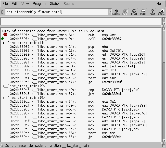
change the syntax to the more familar Intel variety, go to Edit->Gdb
Settings... under Disassembly flavor. This can also be accomplished
with set disassembly-flavor intel from the gdb
prompt. But using the DDD menus will save your settings for future
sessions.
Viewing Memory and the Stack
In gdb, we can easily view the stack by using the x
command. x stands for Examine Memory, and takes the syntax
x /<Number><format letter><size letter>
<ADDRESS>. Format letters are (octal), x(hex),
d(decimal), u(unsigned decimal),
t(binary), f(float), a(address), i(instruction), c(char) and
s(string). Size letters are b(byte), h(halfword), w(word), g(giant, 8
bytes). For example, x /32xw 0x400000 will dump 32
words (32 bit integers) starting at 0x400000. Note that you can also
use registers in place of the address, if you prefix them with a $.
For example, x /32xw $esp will view the top 32
words on the stack.
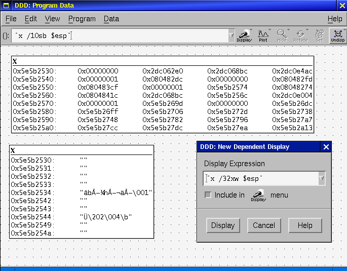
DDD has some nice capabilities for viewing arbitrary dumps of memory
relating to the registers. Go to View->Data Window... Once the Data
Window is open, go to Display (hold down the mouse button as you
click), and go to Other.. You can type in any symbol, variable,
expression, or gdb command (in backticks) in this window, and it will be updated every
time you issue a command to the debugger. A couple good ones to do
would be `x /32xw $esp` and `x/16sb
$esp. Click the little radio button to add these to the menu, and you can then open the stack
from this display and it will be updated in real time as you step
through your program.
Viewing Memory as Specific Data Structures
So DDD has fantastic ability to lay out data structures graphically,
also trough the Display window mentioned above. Simply cast a memory
address to a pointer of a particular type, and DDD will plot the
structure in its graph window. If the data structure contains any
pointers, you can click on these and DDD will open up a display for that
structure as well.
Oftentimes, programs we're interested in won't have any debugging
symbols, and as such, we won't be able to view any structures in an
easy to understand form. For seldom used structures, this isn't that
big of a deal, as you can just take them apart using the
x command. However, if you are dealing with more
complicated data structures, you may want to have a set of types
available to use again and again. Luckily, through the magic of the ELF
format, this is relatively easy to achieve. Simply define whatever
structures or classes you suspect are used and include whatever
headers you
require in a .c file, and then compile it with
gcc -shared. This will produce a .so file. Then,
from within gdb but before you begin debugging, run the command
set env LD_PRELOAD=file.so. From then on, you will
be able to use these types in that gdb/DDD session as if they were
compiled in to the program itself.
(FIXME: Come up with a good example for this).
-> Example using gdb to set breakpoints in functions with and without
debugging symbols.
-> FIXME: Test watchpoints
WinDbg is part of the standart Debugging Tools for Microsoft Windows that
everyone can
download for free from. Microsoft offers few different
debuggers, which use common commands for most operations and ofcourse
there are cases where they differ. Since WinDbg is a GUI program,
all operations are supposed to be done using the provided visual
components. There is also a command line embeded in the debugger,
which lets you type commands just like if you were to use a console
debugger like ntsd. The following section briefly
mentions what commands are used to do common everyday tasks. For more
complete documentation check the Help file that comes with
WinDbg. An example debugging session is
presented to help clarify the usage of the most common commands.
Breakpoints can be set, unset, or listed with the GUI by using
-> or the shortcut keys Alt+F9.
From the command line one can set breakpoints using the
bp command, list them using
bl command, and delete them using
bc command. One can set breakpoints both on
function names (provided the symbol files are available) or on a
memory address. Also if source file is available the debugger will
let you set breakpoints on specific lines using the format
bX `filename:linenumber`
In WinDbg you can use
->
option to open a window which will show you the disassembly of
the current context. In ntsd you can use
the u to view the disassembled code.
There are couple of things one usually does with the stack. One
is to view the frames on the stack, so it can be determined
which function called which one and what is the current context.
This is done using the k command and its
variations. The other common operation is to view the elements
on the stack that are part of the current stack frame. The
easiest way to do so is using db esp ebp, but
it has its limitations. It assumes that the %ebp register
actually points to the begining of the stack frame. This is not
always true, since omission of the frame pointer is common
optimization technique. If this is the case, you can always see
what the %esp register is pointing to and start examining memory
from that address.
The debugger also allows you to "walk" the stack. You can move
to any stack frame using .frame X where X is
the number of the frame. You can easily get the frame numbers
using kn. Keep in mind that the frames are
counted starting from 0 at the frame on top of the stack.
Reading and Writing to Memory
Reading memory is accomplished with the d*
commands. Depending on how you want to view the data you use a
specific variation of this command. For example to see the address
to which a pointer is pointing, we can use dp or
to view the value of a word, one can use dw. The
help file says that one can view memory using ranges, but one can
also use lengths to make it easy to display memory. For example if
we want to see 0x10 bytes at memory location 0x77f75a58 you can
either say db 77f75a58 77f75a58+10 or less
typing gives you db 77f75a58 l 10.
Provided that you have symbols/source files, the
dt is very helpful. It tries to find the data
type of the sybol or memory location and display it accordingly.
Knowing your debugger can save you lots of time and pain in
debugging either your own programs or when reverse engineering
other's. Here are few things we find useful and time saving. This
is not a complete list at all. If you know other tricks and want
to contribute, let us know.
poi() - this command dereferences a pointer to
give you the value that it is pointing to. Using this with
user-defined aliases gives you convinient way of viewing data.
FIXME: include better example Let's set a breakpoint in on the function main
0:000> bp main
*** WARNING: Unable to verify checksum for test.exe
Let's set a breakpoint in on the function main
0:000> g
Breakpoint 0 hit
eax=003212e8 ebx=7ffdf000 ecx=00000001 edx=7ffe0304 esi=00000a28 edi=00000000
eip=00401010 esp=0012fee8 ebp=0012ffc0 iopl=0 nv up ei pl zr na po nc
cs=001b ss=0023 ds=0023 es=0023 fs=0038 gs=0000 efl=00000246
test!main:
00401010 55 push ebp
Enable loading of line information if available
0:000> .lines
*** ERROR: Symbol file could not be found. Defaulted to export symbols for ntdll.dll -
Line number information will be loaded
Set the stepping to be by source lines
0:000> l+t
Source options are 1:
1/t - Step/trace by source line
Enable displaying of source line
0:000> l+s
Source options are 5:
1/t - Step/trace by source line
4/s - List source code at prompt
Start stepping through the program
0:000> p
*** WARNING: Unable to verify checksum for test.exe
eax=003212e8 ebx=7ffdf000 ecx=00000001 edx=7ffe0304 esi=00000a28 edi=00000000
eip=00401016 esp=0012fed4 ebp=0012fee4 iopl=0 nv up ei pl nz na po nc
cs=001b ss=0023 ds=0023 es=0023 fs=0038 gs=0000 efl=00000206
> 6: char array [] = { 'r', 'e', 'v', 'e', 'n', 'g' };
test!main+6:
00401016 c645f072 mov byte ptr [ebp-0x10],0x72 ss:0023:0012fed4=05
0:000>
eax=003212e8 ebx=7ffdf000 ecx=00000001 edx=7ffe0304 esi=00000a28 edi=00000000
eip=0040102e esp=0012fed4 ebp=0012fee4 iopl=0 nv up ei pl nz na po nc
cs=001b ss=0023 ds=0023 es=0023 fs=0038 gs=0000 efl=00000206
> 7: int intval = 123456;
test!main+1e:
0040102e c745fc40e20100 mov dword ptr [ebp-0x4],0x1e240 ss:0023:0012fee0=0012ffc0
0:000>
eax=003212e8 ebx=7ffdf000 ecx=00000001 edx=7ffe0304 esi=00000a28 edi=00000000
eip=00401035 esp=0012fed4 ebp=0012fee4 iopl=0 nv up ei pl nz na po nc
cs=001b ss=0023 ds=0023 es=0023 fs=0038 gs=0000 efl=00000206
> 9: test = (char*) malloc(strlen("Test")+1);
test!main+25:
00401035 6840cb4000 push 0x40cb40
0:000>
eax=00321018 ebx=7ffdf000 ecx=00000000 edx=00000005 esi=00000a28 edi=00000000
eip=00401051 esp=0012fed4 ebp=0012fee4 iopl=0 nv up ei pl nz na po nc
cs=001b ss=0023 ds=0023 es=0023 fs=0038 gs=0000 efl=00000206
> 10: if (test == NULL) {
test!main+41:
00401051 837df800 cmp dword ptr [ebp-0x8],0x0 ss:0023:0012fedc=00321018
0:000>
eax=00321018 ebx=7ffdf000 ecx=00000000 edx=00000005 esi=00000a28 edi=00000000
eip=00401061 esp=0012fed4 ebp=0012fee4 iopl=0 nv up ei pl nz na po nc
cs=001b ss=0023 ds=0023 es=0023 fs=0038 gs=0000 efl=00000206
> 13: strncpy(test, "Test", strlen("Test"));
test!main+51:
00401061 6848cb4000 push 0x40cb48
0:000>
eax=00321018 ebx=7ffdf000 ecx=00000000 edx=74736554 esi=00000a28 edi=00000000
eip=00401080 esp=0012fed4 ebp=0012fee4 iopl=0 nv up ei pl nz ac po nc
cs=001b ss=0023 ds=0023 es=0023 fs=0038 gs=0000 efl=00000216
> 14: test[4] = 0x00;
test!main+70:
00401080 8b4df8 mov ecx,[ebp-0x8] ss:0023:0012fedc=00321018
0:000>
eax=00321018 ebx=7ffdf000 ecx=00321018 edx=74736554 esi=00000a28 edi=00000000
eip=00401087 esp=0012fed4 ebp=0012fee4 iopl=0 nv up ei pl nz ac po nc
cs=001b ss=0023 ds=0023 es=0023 fs=0038 gs=0000 efl=00000216
> 16: printf("Hello RevEng-er, this is %s\n", test);
test!main+77:
00401087 8b55f8 mov edx,[ebp-0x8] ss:0023:0012fedc=00321018
Display the array as bytes and ascii
0:000> db array array+5
0012fed4 72 65 76 65 6e 67 reveng
View the type and value of intval
0:000> dt intval
Local var @ 0x12fee0 Type int
123456
View the type and value of test
0:000> dt test
Local var @ 0x12fedc Type char*
0x00321018 "Test"
View the memory test points to manually
0:000> db 00321018 00321018+4
00321018 54 65 73 74 00 Test.
Quit the debugger
0:000> q
quit:
Unloading dbghelp extension DLL
Unloading exts extension DLL
Unloading ntsdexts extension DLL
Chapter 8. Executable formats| Revision History |
|---|
| Revision $Revision: 1.6 $ | $Date: 2004/01/31 20:56:53 $ | |
So at this point we now know how to write our programs on an extremely
low level, and thus produce an executable file that very closely matches
what we want. But the question is, how is our program code now actually
stored on disk?
We'll begin our investigation into executable formats by looking at the
ELF binary specification and related tools, and then move on to
examine the PE binary
specification, and related tools for dealing with those binaries.
Working with the ELF Program FormatRecall that when a Linux program runs, we start at the _start
function,
and move on from there to __libc_start_main, and eventually to main, which
is our code. So somehow the operating system is gathering together a whole
lot of code from various places, and loading it into memory and then
running it. How does it know what code goes where? The answer on Linux and UNIX is the
ELF binary specification. ELF specifies a standard format for
mapping your code on disk to a complete executable image in
memory that consists of your code, a stack, a heap (for malloc), and all
the libraries you link against. So lets provide an overview of the information needed for our purposes
here, and refer the user to the ELF spec to fill in the details if they
wish. We'll start from the beginning of a typical executable and work our
way down. There are three header areas in an ELF file: The main ELF file header,
the program headers, and then the section headers. The program code lies
in between the program headers and the section headers. TODO: Insert figure here to show a typical ELF layout. NOTE: ELF is extremely flexible. Many of these sections can be shunk,
expanded, removed, etc. In fact, it is not outside the realm of
possibility that some programs may deliberately make abnormal, yet valid
ELF headers and files to try to make reverse engineering difficult
(vmware does this, for example). The main elf header basically tells us where everything is located in
the file. It comes at the very beginning of the executable, and can be
read directly from the first e_ehsize (default: 52) bytes of the file
into this structure. /* ELF File Header */
typedef struct
{
unsigned char e_ident[EI_NIDENT]; /* Magic number and other info */
Elf32_Half e_type; /* Object file type */
Elf32_Half e_machine; /* Architecture */
Elf32_Word e_version; /* Object file version */
Elf32_Addr e_entry; /* Entry point virtual address */
Elf32_Off e_phoff; /* Program header table file offset */
Elf32_Off e_shoff; /* Section header table file offset */
Elf32_Word e_flags; /* Processor-specific flags */
Elf32_Half e_ehsize; /* ELF header size in bytes */
Elf32_Half e_phentsize; /* Program header table entry size */
Elf32_Half e_phnum; /* Program header table entry count */
Elf32_Half e_shentsize; /* Section header table entry size */
Elf32_Half e_shnum; /* Section header table entry count */
Elf32_Half e_shstrndx; /* Section header string table index */
} Elf32_Ehdr;
The fields of interest to us are e_entry, e_phoff, e_shoff, and the
sizes given. e_entry specifies the location of _start, e_phoff shows us
where the array of program headers lies in relation to the start of the
executable, and e_shoff shows us the same
for the section headers.
The next portion of the program are the ELF program headers. These
describe the sections of the program that contain executable program
code to get mapped into the program address space as it loads. /* Program segment header. */
typedef struct
{
Elf32_Word p_type; /* Segment type */
Elf32_Off p_offset; /* Segment file offset */
Elf32_Addr p_vaddr; /* Segment virtual address */
Elf32_Addr p_paddr; /* Segment physical address */
Elf32_Word p_filesz; /* Segment size in file */
Elf32_Word p_memsz; /* Segment size in memory */
Elf32_Word p_flags; /* Segment flags */
Elf32_Word p_align; /* Segment alignment */
} Elf32_Phdr;
Keep in mind that there are going to a few of these (usually 2)
end-to-end (ie forming an array of structs) in a typical ELF executable.
The interesting fields in this structure are
p_offset, p_filesz, and p_memsz, all of which we will need to make use of in the
code modification chapter. The meat of the ELF file comes next. The actual locations and sizes
of portions of the body are described by the
program headers above, and contain the executable instructions from our
assembly file, as well as string constants and global variable
declarations.
The ELF section headers describe various named sections in an executable
file. Each section has an entry in the section headers array, which is
found at the bottom of the executable and has the following
format: /* Section header. */
typedef struct
{
Elf32_Word sh_name; /* Section name (string tbl index) */
Elf32_Word sh_type; /* Section type */
Elf32_Word sh_flags; /* Section flags */
Elf32_Addr sh_addr; /* Section virtual addr at execution */
Elf32_Off sh_offset; /* Section file offset */
Elf32_Word sh_size; /* Section size in bytes */
Elf32_Word sh_link; /* Link to another section */
Elf32_Word sh_info; /* Additional section information */
Elf32_Word sh_addralign; /* Section alignment */
Elf32_Word sh_entsize; /* Entry size if section holds table */
} Elf32_Shdr;
The section headers are entirely optional, however. A list of
common sections can be found on page 20 of the ELF Spec
PDF Editing ELF is often desired during reverse engineering, especially
when we want to insert bodies of code, or if we want to reverse engineer
binaries with deliberately corrupted ELF headers. Now you could edit these headers by hand using the <elf.h> header
file and those above structures, but luckily there is already a nice
editor called HT Editor
that allows you to examine and modify
all sections of an ELF program, from ELF header to actual
instructions.
(TODO: instructions, screenshots of HTE)
Do note that changing the size of various program sections in the ELF
headers will most likely break things. We will get into how to edit ELF
in more detail when we are talking about actual code insertion, which is
the next chapter.
FIXME: Describe what ELF looks like in memory on Linux (and maybe xBSD
and Solaris). Include memory addresses and diagrams of the process space.
Working with the PE Program Format
Unfortunately, the PE format can be a bit of a maze, so we're only going to
discuss those sections relevant to code modification, namely the Import
Address Table and code sections. FIXME: what is the equiv of _start for
Microsoft Windows.
FIXME: How does COM use its directory entry?
So lets start with some basic concepts. There are essentially four ways to
refer to a location in a PE image (and all are used by the various data
structures in some form or another).
Executable File Offset
This is simply the offset from the beginning of the executable file.
Relative Virtual Address (RVA)
This is the offset from the base address of the executable image
once it has been mapped into memory. Note that this is
not the same as the executable file offset.
Various sections within the executable file have to start on page
aligned boundaries, and as a result, holes must be present in memory
that are not present in the disk image. This is a big source of
confusion when initially working with PE's.
Section Offset
This is the offset from whatever data structure or section you are
currently in. Yes, in some cases it is used in lieu of the RVA.
(FIXME: Build a semi-complete list of these).
Virtual Address
This is a full pointer into the address space of the process.
Virtual addresses can be obtained by the formula VA = RVA + base
address .
For almost all executables, the base address is 0x400000. For DLL's,
the base address can vary, as the address requested by the DLL in its
header is much more likely to conflict with another DLL. The
accompanying source code (FIXME: Clean up and Link in) for function
injection contains a function that converts RVA's to VA's or file
offsets, depending upon the context.
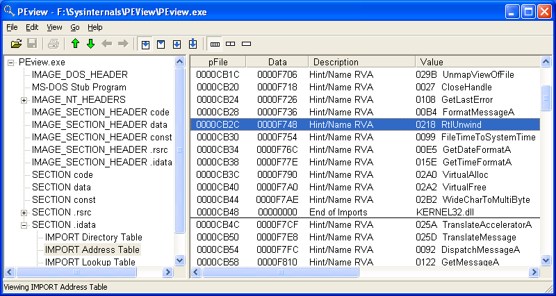
So there are three main header types to a PE file. It's going to be a lot to keep track of. Luckily, the PEView utility
can make things much more easy to understand. We suggest using it on an
executable and following along so you don't get lost. These headers and
the supporting macros are all defined in WinNT.h in the PlatformSDK
include directory.
The first is the IMAGE_DOS_HEADER. It is at file offset and RVA 0.
The IMAGE_DOS_HEADER is a relic from the (you guess it) DOS days. It's
only function now the e_lfanew field, which gives the offset to the of
the IMAGE_NT_HEADERS structure, which is where the real action starts.
Technically this is a file offset, but at this point, allignment isn't
an issue, and it can be intrepreted as an RVA as well. One other thing
to note: e_magic has the value IMAGE_DOS_HEADER, which is "MZ" or
0x5A4D.
Next up on the chopping block is the IMAGE_NT_HEADERS:
Not really much of interest at this level. That Signature field is just
to make sure you're in the right place, and has the value
IMAGE_NT_SIGNATURE, which is PE00, or 0x00004550. If we open up that
IMAGE_FILE_HEADER:
This essentially is only useful (for our purposes) for knowing the
number of sections and the size of the optional header (which isn't
very optional). The optional header size is needed because there can be
a varying number of directory entries in the header, and this size is
used to find the start of the section table (with the
IMAGE_FIRST_SECTION() macro).
So the interesting fields here are ImageBase, AddressOfEntryPoint,
SectionAlignment, and the CheckSum (FIXME: do they ever use this?).
After that comes the DataDirectory, which contains basicaly the root of an
entire filesystem heirarchy within the executable. Luckily most executables
only use the top level of this filesystem.
So the array of these is what makes up the end of the optional header.
Don't be fooled by that name, it is in fact a relative virtual address.
Lets have a look at the data structure for the second array index (ie
index 1). Going to this RVA will take us to the import directory, which
is an array of DLL's that this PE file is linked against.
So these fields can be a bit confusing, mostly because at this point, the PE
format itself gets a bit confusing. First off, the OriginalFirstThunk is an
RVA, as is Name and FirstThunk. So this is important. Name isn't a pointer to
an ASCII string, but an RVA to one, which you must convert. The last import
descriptor in the file will have zeroes for all of its fields and it serves
as an end marker.
As the comments indicate, there are in fact two import tables for each DLL.
When non-zero, OriginalFirstThunk refers to the "Unbound" Import Table.
FirstThunk, on the other hand, refers to the Import Address Table.
One data structure describes both of these import tables:
In many executables files, both of these tables look exactly the same. The
reason for this is that the IAT is rewritten when the executable is loaded into
memory, and at that point contains the actual addresses of imported functions
(hence the Function member of the union). It then servers a purpose similar to
the PLT we saw in the ELF format. As the name OriginalThunk suggests, the
"Unbound" Import Table remains unchanged, to preserve function name and ordinal
information (to what end, no one seems to really know. FIXME: Maybe LoadLibrary
uses this to remap functions if DLL's need to be shuffled around?). In some
executables, the IAT can come pre-bound, and filled in with expected addresses
already as an efficiency mechanism.
But, the complexities don't end there. An imported function can be listed by
name, or it can be listed by an ordinal number which represents its position in
the DLL's export table. If it is listed by an ordinal number, high bit
(1<<31, or 0x80000000) of this union is set. If it is not set, then it is
either an RVA to a forwarder string, a function address (which is a Virtual
Address), or an RVA to a structure that contains the function name (FIXME: How
are these three differentiated?)
So there's quite a bit more to the PE format than we discussed here.
Luckly, most
if it isn't directly relevant. Our ticket to paradise is that Function
member field of the Import Address Table. Modifying him will allow us to
drop in any old arbitrary function we want, as we will cover in the Code modification Chapter. Things you might want to cover
if you're curious are the export tables and the COM data directory.
(FIXME: Consider documenting COM tables).
FIXME: Describe what PE looks like in memory. Include memory addresses,
and a diagram of process space.
Chapter 9. Code Modification
So now we know the tools to analyze our programs and find functions of
interest to us even in programs without source code. We can understand
the assembly
that makes them up, and can write assembly of our own to do what we want.
We know how a program looks on the disk and how that corresponds to what
the program looks like in memory. Knowledge is power, and we know a lot.
Reasons for Code Modification
Code modification is most useful if we wish to change the behavior of
programms for which we do not have source code on hand. It is also
handy when trying to skirt copy protection of various kinds.
This is an environment variable that allows us to add a library to the
execution of a particular program. Any functions in this library
automatically override standard library functions. Sorry, you can't use
this with suid programs.
Example: % gcc -o preload.so -shared preload.c -ldl % LD_PRELOAD=preload.so ssh students.uiuc.edu
Since the smallest unit of code is the instruction, it follows that
the simplest form of code modification is instruction modification.
In instruction modification, we are looking to change some property of a
specific instruction. Recall from the assembly section that each
instruction has 2 parts: The mnemonic and the arguments. So our choices
are limited.
The best way to modify instructions is through HT Editor, which was mentioned
earlier in the ELF section. HTE has a hex editor mode where we can edit
the hex value of an instruction and see the assembly updated in real time.
(TODO: instructions, screenshots of HTE)
Editing the arguments of an assembly instruction is easy. Simply look
at the hex value of the assembly instruction's argument, and see where
it lies in the hex bytes for that instruction. HTE will allow you to
overwrite these values with values of your own.
(Be careful with byte ordering!).
TODO: Example1.
Single Instruction InsertionSingle Function InsertionUse unused space as found by disasm.pl (be careful about main)
Multiple Function InsertionTrickery.. We're working on a util to modify ELF programs and insert
functions. What about using MMAP?? (P.S. Can you unmap executable
memory to modify it... if they are doing an MD5 of their
executable) Attacking copy protectionLest I be accused of hiding in my ivory tower, lets look a
concrete application of these ideas, and some techniques (: Chapter 12. Extra Resources| Revision History |
|---|
| Revision $Revision: 1.3 $ | $Date: 2004/01/31 20:56:53 $ | |
Other Resources and amusements
LDasm project. LDasm is at best a passable disassembly tool
(disasm.pl is FAR more useful), but it does come with a utility called
ptrace, which allows you to view which instructions of a program
actually execute. You can also give ptrace a list of addresses (for
example, the list of functions found by disasm.pl) and have it step
through those to show you which ones actually execute in your
program.
Creating Teensy Executables in Linux
Microsoft COFF format
Attacking FlexLM is an essay written in 1998 on attacking a specific form of
hard copy protection. There are several other essays on that site, but most
of them cover material that we cover above, but with specific example
programs.
|

 LINUX
LINUX 
 Books
Books