Search     or:     and:
 LINUX 
 Language 
 Kernel 
 Package 
 Book 
 Test 
 OS 
 Forum 
 iakovlev.org 
 Books
  Краткое описание
 Linux
 W. R. Стивенс TCP 
 W. R. Стивенс IPC 
 A.Rubini-J.Corbet 
 K. Bauer 
 Gary V. Vaughan 
 Д Вилер 
 В. Сталлинг 
 Pramode C.E. 
 Steve Pate 
 William Gropp 
 K.A.Robbins 
 С Бекман 
 Р Стивенс 
 Ethereal 
 Cluster 
 Languages
 C
 Perl
 M.Pilgrim 
 А.Фролов 
 Mendel Cooper 
 М Перри 
 Kernel
 C.S. Rodriguez 
 Robert Love 
 Daniel Bovet 
 Д Джеф 
 Максвелл 
 G. Kroah-Hartman 
 B. Hansen 
NEWS
Последние статьи :
  Тренажёр 16.01   
  Эльбрус 05.12   
  Алгоритмы 12.04   
  Rust 07.11   
  Go 25.12   
  EXT4 10.11   
  FS benchmark 15.09   
  Сетунь 23.07   
  Trees 25.06   
  Apache 03.02   
 
TOP 20
 MINIX...3058 
 Solaris...2934 
 LD...2907 
 Linux Kernel 2.6...2488 
 William Gropp...2187 
 Rodriguez 6...2018 
 C++ Templates 3...1948 
 Trees...1941 
 Kamran Husain...1868 
 Secure Programming for Li...1795 
 Максвелл 5...1712 
 DevFS...1696 
 Part 3...1686 
 Stein-MacEachern-> Час...1635 
 Go Web ...1630 
 Ethreal 4...1620 
 Стивенс 9...1609 
 Arrays...1609 
 Максвелл 1...1598 
 FAQ...1540 
 
  01.01.2024 : 3621733 посещений 

iakovlev.org

Структуры данных

Память , абстрактные типы данных , адреса

Каково максимальное число попыток , которое нужно вам для того , чтобы найти определенное имя в списке из миллиона имен ? Миллион ? Гораздо меньше. Это можно сделать за 20 попыток , если ваш список имеет эффективный алгоритм поиска. Поисковые списки - один из способов структурирования данных , который помогает вам манипулировать этими данными в памяти вашего компьютера В этом разделе вы увидите , как устроена память компьютера , и почему в памяти хранятся только нули и единицы :-)

Обзор памяти

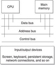
Computer memory is divided into three sections: main memory, cache memory in the central processing unit (CPU), and persistent storage. Main memory, also called random access memory (RAM), is where instructions (programs) and data are stored. Main memory is volatile; that is, instructions and data contained in main memory are lost once the computer is powered down.

Cache memory in the CPU is used to store frequently used instructions and data that either is, will be, or has been used by the CPU. A segment of the CPU’s cache memory is called a register. A register is a small amount of memory within the CPU that is used to temporarily store instructions and data.

A bus connects the CPU and main memory. A bus is a set of etched wires on the motherboard that is similar to a highway and transports instructions and data between the CPU, main memory, and other devices connected to a computer (see Figure 1-1).

Click To expand
Figure 1-1: A bus connects the CPU, main memory, persistent storage, and other devices.

Persistent storage is an external storage device such as a hard disk that stores instructions and data. Persistent storage is nonvolatile; that is, instructions and data remain stored even when the computer is powered down.

Persistent storage is commonly used by the operating system as virtual memory. Virtual memory is a technique an operating system uses to increase the main memory capacity beyond the random access memory (RAM) inside the computer. When main memory capacity is exceeded, the operating system temporarily copies the contents of a block of memory to persistent storage. If a program needs access to instructions or data contained in the block, the operating system switches the block stored in persistent storage with a block of main memory that isn’t being used.

CPU cache memory is the type of memory that has the fastest access speed. A close second is main memory. Persistent storage is a distant third because persistent storage devices usually involve a mechanical process that inhibits the quick transfer of instructions and data.

Throughout this book, we’ll focus on main memory because this is the type of memory used by data structures (although the data structures and techniques presented can also be applied to file systems on persistent storage).

Данные и память

Data used by your program is stored in memory and manipulated by various data structure techniques, depending on the nature of your program. Let’s take a close look at main memory and how data is stored in memory before exploring how to manipulate data using data structures.

Memory is a bunch of electronic switches called transistors that can be placed in one of two states: on or off. The state of a switch is meaningless unless you assign a value to each state, which you do using the binary numbering system.

The binary numbering system consists of two digits called binary digits (bits): zero and one. A switch in the off state represents zero, and a switch in the on state represents one. This means that one transistor can represent one of two digits.

However, two digits don’t provide you with sufficient data to do anything but store the number zero or one in memory. You can store more data in memory by logically grouping together switches. For example, two switches enable you to store two binary digits, which gives you four combinations, as shown Table 1-1, and these combinations can store numbers 0 through 3. Digits are zero-based, meaning that the first digit in the binary numbering system is zero, not 1. Memory is organized into groups of eight bits called a byte, enabling 256 combinations of zeros and ones that can store numbers from 0 through 255.

Table 1-1: Combinations of Two Bits and Their Decimal Value Equivalents

Switch 1

Switch 2

Decimal Value

0

0

0

0

1

1

1

0

2

1

1

3

The Binary Numbering System

A numbering system is a way to count things and perform arithmetic. For example, humans use the decimal numbering system, and computers use the binary numbering system. Both these numbering systems do exactly the same thing: they enable us to count things and perform arithmetic. You can add, subtract, multiply, and divide using the binary numbering system and you’ll arrive at the same answer as if you used the decimal numbering system.

However, there is a noticeable difference between the decimal and binary numbering systems: the decimal numbering system consists of 10 digits (0 through 9) and the binary numbering system consists of 2 digits (0 and 1).

To jog your memory a bit, remember back in elementary school when the teacher showed you how to “carry over” a value from the right column to the left column when adding two numbers? If you had 9 in the right column and added 1, you changed the 9 to a 0 and placed a 1 to the left of the 0 to give you 10:

The same “carry over” technique is used when adding numbers in the binary numbering system except you carry over when the value in the right column is 1 instead of 9. If you have 1 in the right column and add 1, you change the 1 to a 0 and place a 1 to the left of the 0 to give you 10:

Now the confusion begins. Both the decimal number and the binary number seem to have the same value, which is ten. Don’t believe everything you see. The decimal number does represent the number 10. However, the binary number 10 isn’t the value 10 but the value 2.

The digits in the binary numbering system represent the state of a switch. A computer performs arithmetic by using the binary numbering system to change the state of sets of switches.

Chapter 2: The Point About Variables and Pointers

Some programmers cringe at the mere mention of the word “pointer” because it brings to mind complex, low-level programming techniques that are confounding. Hogwash. Pointers are child play, literally. Watch a 15-month-old carefully and you’ll notice that she points to things she wants, and that’s a pointer in a nutshell. A pointer is a variable that is used to point to a memory address whose content you want to use in your program. You’ll learn all about pointer variables in this chapter.

Declaring Variables and Objects

Memory is reserved by using a data type in a declaration statement. The form of a declaration statement varies depending on the programming language you use. Here is a declaration statement for C, C++, and Java:

int myVariable;

There are three parts to this declaration statement:

  • Data type Tells how much memory to reserve and the kind of data that will be stored in that memory location

  • Variable name A name used within the program to refer to the contents of that memory location

  • Semicolon Tells the computer this is an instruction (statement)

Primitive Data Types and User-Defined Data Types

In Chapter 1, you were introduced to the concept of abstract data types, which are used to reserve computer memory. Abstract data types are divided into two categories, primitive data types and user-defined data types. A primitive data type is defined by the programming language, such as the data types you learned about in the previous chapter. Some programmers call these built-in data types.

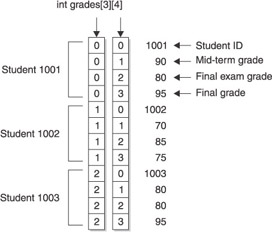
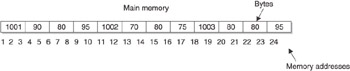
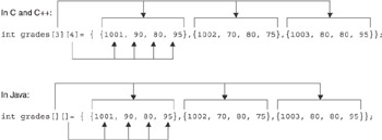
The other category of abstract data type, a user-defined data type, is a group of primitive data types defined by the programmer. For example, let’s say you want to store students’ grades in memory. You’ll need to store 4 data elements: the student’s ID, first name, last name, and grade. You could use primitive data types for each data element, but primitive data types are not grouped together; each exists as separate data elements.

A better approach is to group primitive data types into a user-defined data type to form a record. You probably heard the term “record” used when you learned about databases. Remember that a database consists of one or more tables. A table is similar to a spreadsheet consisting of columns and rows. A row is also known as a record. A user-defined data type defines columns (primitive data types) that comprise a row (a user-defined data type).

The form used to define a user-defined data type varies depending on the programming language used to write the program. Some programming languages, such as Java, do not support user-defined data types. Instead, attributes of a class are used to group together primitive data types; this is discussed later in this chapter.

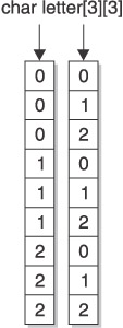
In the C and C++ programming languages, you define a user-defined data type by defining a structure. Think of a structure as a stencil of the letter A. The stencil isn’t the letter A, but it defines what the letter A looks like. If you want a letter A, you place the stencil on a piece of paper and trace the letter A. If you want to make another letter A, you use the same stencil and repeat the process. You can make as many letter A’s as you wish by using the stencil.

The same is true about a structure. When you want the group of primitive data types represented by the structure, you create an instance of the structure. An instance is the same as the letter A appearing on the paper after you remove the stencil.

Each instance contains the same primitive data types that are defined in the structure, although each instance has its own copy of those primitive data types.

Defining a User-Defined Data Type

A structure definition consists of four elements:

  • struct Tells the computer that you are defining a structure

  • Structure name The name used to uniquely identify the structure and used to declare instances of a structure

  • Structure bodypen and close braces within which are primitive data types that are declared when an instance of the structure is declared

  • Semicolon Tells the computer this is an instruction (statement)

The body of a structure can contain any combination of primitive data types and previously defined user-defined data types depending on the nature of the data required by your program. Here is a structure that defines a student record consisting of a student number and grade. The name of this user-defined data type is StudentRecord:

struct StudentRecord
 {
  int studentNumber;
  char grade;
 };

Declaring a User-Defined Data Type

You declare an instance of a user-defined data type using basically the same technique that you used to declare a variable. However, you use the name of the structure in place of the name of the primitive data type in the declaration station.

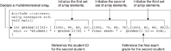
Let’s say that you want to create an instance of the StudentRecord structure defined in the previous section. Here’s the declaration statement that you need to declare in your program:

#include <iostream>
 using namespace std;
 struct StudentRecord
 {
  int studentNumber;
  char grade;
 } ;
 void main()
 {
  StudentRecord myStudent;
  myStudent.studentNumber = 10;
  myStudent.grade = 'A';
  cout << "grades: " << myStudent.studentNumber << " "
  << myStudent.grade << endl;
 }

The declaration statement tells the computer to reserve memory the size required to store the StudentRecord user-defined data type and to associate myStudent with that memory location. The size of a user-defined data type is equal to the sum of the sizes of the primitive data types declared in the body of the structure.

The size of the StudentRecord user-defined data type is the sum of the sizes of an integer and a char. As you recall from Chapter 1, the size of a primitive data type is measured in bits. The number of bits for the same primitive data type varies depending on the programming language. Therefore, programmers refer to the name of the primitive data type rather than the number of bits when reserving memory. The computer knows how many bits to reserve for each primitive data type.

User-Defined Data Types and Memory

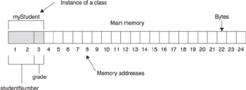
Data elements within the body of a structure are placed sequentially in memory when an instance of the structure is declared within a program. Figure 2-1 illustrates memory reserved when the myStudent instance of StudentRecord is declared.

Click To expand
Figure 2-1: Memory for elements of a structure are placed in sequential memory locations when an instance of the structure is declared.

The instance name myStructure is an alias for the memory address that is reserved for the first primitive data type defined in the StudentRecord structure, which is memory address 1 in Figure 2-1. For the sake of simplicity, let’s say each block shown in Figure 2-1 represents 1 byte of memory and the size of an int is 2 bytes.

Each primitive data type of a structure has its own memory address. The first primitive data type in this example is studentNumber, and its name references memory location 1. The second primitive data type is grade, and its name references memory location 2.

What happened to memory location 1? This can be confusing. Remember that each byte of memory is assigned a unique memory address. Some primitive data types are larger than a byte and therefore must occupy more than one memory address, which is the case in this example with an int. The first primitive data type takes up the first 2 bytes of memory. Therefore, the second primitive data type defined in the structure is placed in the next available byte of memory, which is memory location 2.

Accessing Elements of a User-Defined Data Type

Elements of a data structure are accessed by using the name of the instance of the structure and the name of the element separated by a dot operator. Let’s say that you want to assign the grade A to the grade element of the myStudent instance of the StudentRecord structure. Here’s how you would write the assignment statement:

myStudent.grade = 'A';

You use elements of a structure the same way you use a variable within your program except you must reference both the name of the instance and the name of the element in order to access the element. The combination of instance name and element name is the alias for the memory location of the element.

User-Defined Data Type and Classes

Structures are used in procedure languages such as C. Object-oriented languages such as C++ and Java use both structures and classes to group together unlike primitive data types into a cohesive unit.

A class definition is a stencil similar in concept to a structure definition in that both use the definition to create instances. A structure definition creates an instance of a structure, while a class definition creates an instance of a class.

A class definition translates attributes and behaviors of a real life object into a simulation of that object within a program. Attributes are data elements similar to elements of a structure. Behaviors are instructions that perform specific tasks known as either methods or functions, depending on the programming language used to write the program. Java references these as methods and C++ references them as functions.

Defining a Class

A class definition resembles a definition of a structure, as you can see in the following example. A class definition consists of four elements:

  • class Tells the computer that you are defining a class

  • Class name The name used to uniquely identify the class and used to declare instances of a class

  • Class body Open and close braces within which are primitive data types that are declared when an instance of the class is declared and definitions

  • of methods and functions that are members of the class

  • Semicolon Tells the computer this is an instruction (statement)

The following class definition written in C++ defines the same student record that is defined in the structure defined in the previous section of this chapter. However, the class definition also defines a function that displays the student number and grade on the screen.

class StudentRecord {
  int studentNumber;
  char grade;
  void displayGrade() {
  cout<<"Student: " << studentNumber << " Grade: "
  << grade << endl;
  }
 };

Declaring an Instance of a Class and a Look at Memory

You declare an instance of a class much the same way you declare a structure. That is, you use the name of the class followed by the name of the instance of the class in a declaration statement. Here is how an instance of the StudentRecord class is declared:

StudentRecord myStudent;
 

Memory is reserved for attributes of a class definition sequentially when an instance is declared, much the same way as memory is reserved for elements of a structure. Figure 2-2 shows memory allocation for the myStudent instances of the StudentRecord class. Notice that this is basically the same way memory for a structure is allocated.

Click To expand
Figure 2-2: Memory for attributes of a class are placed in sequential memory locations when an instance of the class is declared.

Methods and functions are stored separately in memory from attributes when an instance is declared because methods and functions are shared among all instances of the same class.

Accessing Members of a Class

Attributes, methods, and functions are referred to as members of a class. You access members of an instance of a class using the name of the instance, the dot operator and the name of the member, much the same ways as you access an element of a structure.

Here is how to access the grade attribute of the myStudent instance of the StudentRecord class and call the displayGrade() method:

myStudent.grade = 'A';
 myStudent.displayGrade();

Pointers

Whenever you reference the name of a variable, the name of an element of a structure, or the name of an attribute of a class, you are telling the computer that you want to do something with the contents stored at the corresponding memory location.

In the first statement in the following example, the computer is told to store the letter A into the memory location represented by the variable grade. The last statement tells the computer to copy the contents of the memory location represented by the grade variable and store it in the memory location represented by the oldGrade variable.

char grade = 'A';
 char oldGrade;
 oldGrade = grade;

A pointer is a variable and can be used as an element of a structure and as an attribute of a class in some programming languages such as C++, but not Java. However, the contents of a pointer is a memory address of another location of memory, which is usually the memory address of another variable, element of a structure, or attribute of a class.

Declaring a Pointer

A pointer is declared similar to how you declare a variable but with a slight twist. The following example declares a pointer called ptGrade. There are four parts of this declaration:

  • Data type The data type of the memory address stored in the pointer

  • Asterisk (*) Tells the computer that you are declaring a pointer

  • Variable name The name that uniquely identifies the pointer and is used to reference the pointer within your program

  • Semicolon Tells the computer this is an instruction (statement)

    char *ptGrade;

Data Type and Pointers

As you will recall, a data type tells the computer the amount of memory to reserve and the kind of data that will be stored at that memory location. However, the data type of a pointer tells the computer something different. It tells the computer the data type of the value at the memory location whose address is contained in the pointer.

Confused? Many programmers are confused about the meaning of the data type used to declare a pointer, so you’re in good company. The best way to clear any confusion is to get back to basics.

The asterisk (*) used when declaring a pointer tells the computer the amount of memory to reserve and the kind of data that will be stored at that location. That is, the memory size is sufficient to hold a memory address, and the kind of data stored there is a memory address.

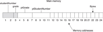
You’re probably wondering why you use a data type when declaring a pointer. Before answering that question, let’s make sure you have a firm understanding of pointers. The following example declares four variables. The first statement declares an integer variable called studentNumber. The second statement declares a char variable called grade. The last two statements each declare a pointer. Figure 2-3 depicts memory reserved by these statements. Assume that a memory address is 4 bytes for this example.

Click To expand
Figure 2-3: Memory allocated when two pointers and two variables are declared
int studentNumber;
 char grade;
 char *ptGrade;
 int *ptStudentNumber;

The char data type in the ptGrade pointer declaration tells the computer that the address that will be stored in ptGrade is the address of a character. As you’ll see in the next section, the contents of the memory location associated with ptGrade will contain the address of the grade variable.

Likewise, the int data type of the ptStudentNumber pointer states that the contents of the memory location associated with ptStudentNumber will contain the address of an integer variable, which will be the address of the studentNumber variable.

Why does the computer need to know this? For now, let’s simply say that programmers instruct the computer to manipulate memory addresses using pointer arithmetic. In order for the computer to carry out those instructions, the computer must know the data type of the address contained in a pointer. You’ll learn pointer arithmetic later in this chapter.

Assigning an Address to a Pointer

An address of a variable is assigned to a pointer variable by using the address operator (&). Before you learn about dereferencing a variable, let’s review an assignment statement. The following assignment statement tells the computer to copy the value stored at the memory location that is associated with the grade variable and store the value into the memory location associated with the oldGrade variable:

oldGrade = grade;

An assignment statement implies that you want the contents of a variable and not the address of the variable. The address operator tells the computer to ignore the implied assignment and assign the memory address of the variable and not the content of the variable.

The next example tells the computer by using the address operator to copy the address of the variable to the pointer variable. That is, the memory address of the grade variable is copied to the ptGrade pointer variable, and the memory address of the studentNumber variable is assigned to the ptStudentNumber pointer:

ptGrade = &grade;
 ptStudentNumber = &studentNumber;

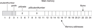
Figure 2-4 depicts memory after the previous two statements execute. Notice that the grade variable is an alias for memory address 3 and the studentNumber variable is the alias for memory address 1. The content of ptGrade pointer is 3, which is the memory address of the grade variable. Likewise, the content of pointer ptStudentNumber is 1, which is the memory address of studentNumber.

Click To expand
Figure 2-4: Memory allocated after pointers are assigned memory addresses

Accessing Data Pointed to by a Pointer

A pointer variable references a memory location that contains a memory address. Sometimes a programmer wants to copy that memory address to another pointer variable. This is accomplished by using an assignment statement as shown here:

ptOldGrade = ptNewGrade;

You’ll notice that this assignment statement is identical to assignment statements used with any variable. Remember that the assignment statement tells the computer to copy the contents of a variable regardless if the content is a memory address or any other value.

Other times, programmers want to the use the content of the memory address stored in the pointer variable. This may be tricky to understand, so let’s look at an example to clear up any confusion. The following statements will be familiar to you because we’ve used them in examples throughout this chapter.

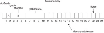
The first two statements declare variables, one of which is initialized with a value. The next two statements declare pointer variables. And the last statement assigns the address of the first variable to pointer variables. Figure 2-5 shows how memory looks after these statements execute.

Click To expand
Figure 2-5: Memory allocated after values are assigned to variables
char oldGrade;
 char grade = 'A';
 char *ptGrade;
 char *ptOldGrade;
 ptGrade = &grade;

Let’s say a programmer wants to use the value stored in the grade variable to display the grade on the screen. However, the programmer wants to use only the ptGrade pointer to do this. Here’s how it is done.

The programmer uses the pointer dereferencing operator (sometimes called the dereferencing operator), which is the asterisk (*), to dereference the point variable. Think of dereferencing as telling the computer you are referring to to go to the memory address contained in the pointer and then perform the operation. Without dereferencing, the computer is told to use the contents of the pointer when performing the operation.

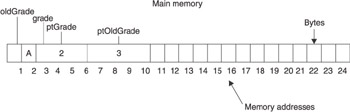
Let’s say that you want to copy the content of ptGrade to ptOldGrade. Here’s how you would do it:

ptOldGrade = ptGrade;

Figure 2-6 shows you the effect this statement has on memory.

Click To expand
Figure 2-6: Memory allocated after the value of the ptGrade is copied to ptOldGrade.

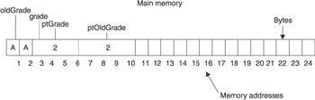
Now let’s suppose you want to copy the contents of grade to the oldGrade variable, but you only want to use the ptGrade pointer. You do this by dereferencing the ptGrade pointer variable using the asterisk (*) as the dereferencing pointer operator as shown here:

char oldGrade = *ptGrade;

The previous statement tells the computer to go to the memory address contained in the ptGrade pointer variable and then perform the assignment operation, which copies the value of memory address 2 to the memory address represented by the oldGrade variable, which is memory address 1. The result is shown in Figure 2-7.

Click To expand
Figure 2-7: Memory allocated after the contents of the memory address pointed to by ptGrade is copied to the oldGrade variable.

You can dereference a pointer variable any time you want to use the contents of the memory address pointed to by the variable and use the dereference pointer variable in any statement that you would use a variable.

Pointer Arithmetic

Pointers are used to step through memory sequentially by using pointer arithmetic and the incremental (++) or decremental (- -) operator. The incremental operator increases the value of a variable by 1, and the decremental operator decreases the value of a variable by 1.

In the following example, the value of the studentNumber variable is incremented by 1, making the final value 1235.

int studentNumber = 1234;
 studentNumber++;

Likewise, the next example decreases the value of the studentNumber variable by 1, resulting in the final value of 1233.

int studentNumber = 1234;
 studentNumber--;

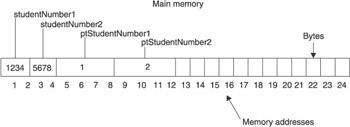
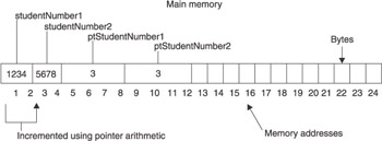
Pointer arithmetic uses the incremental and decremental operator in a similar but slightly different way. The following statements declare two variables used to store student numbers and two pointers each pointing to one of those variables. Figure 2-8 depicts memory allocation after these statements execute.

Click To expand
Figure 2-8: Memory allocation before incrementing ptStudentNumber1
int studentNumber1 = 1234;
 int studentNumber2 = 5678;
 int *ptStudentNumber1;
 int *ptStudentNumber2;
 ptStudentNumber1 = &studentNumber1;
 ptStudentNumber2 = &studentNumber2;
 

What would be the value stored in the pointer variable studentNumber1 if the studentNumber1 is incremented by 1 using the following statement?

ptStudentNumber1++;

This is tricky because the value of ptStudentNumber1 is 0. If you increment it by one, the new value is 1. However, memory address 2 is the second half of the memory location reserved for studentNumber1. This means that ptStudentNumber1 would point to the middle of the values of studentNumber1, which doesn’t make sense.

That’s not what happens. The computer uses pointer arithmetic. Values are incremented and decremented in pointer arithmetic using the size of a data type. That is, if the memory address contains an integer and the memory address is incremented, the computer adds the size of an integer to the current memory address.

Let’s return to Figure 2-8 and see how this works. ptStudentNumber1 contains the memory address 1. If you go to memory address 1, you’ll notice that the memory address stores an integer. In the example, the size of an integer is 2 bytes. When ptStudentNumber1 is incremented using pointer arithmetic, the computer adds 2 bytes to the address stored in ptStudentNumber1 making the new value 2, which is stored in ptStudentNumber1. Figure 2-9 shows the results of incrementing using pointer arithmetic.

Click To expand
Figure 2-9: Memory allocation after incrementing ptStudentNumber1

Decrementing a value using pointer arithmetic is very similar to incrementing a value, except the size of a data type is subtracted from the value. Let’s return to Figure 2-8 for a moment. If the following statement executed, the value of ptStudentNumber2 would be 1 because the computer subtracts the size of an integer (2 bytes) from the current value of the ptStudentNumber2 (2).

ptStudentNumber2--;

Pointers to Pointers

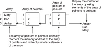
Imagine having a list of a million students along with their final grades and student numbers and being asked to sort the list by last name, first name, and student number. Intuitively, you might think about making two copies of this list, each placed in one of the sort orders. However, this wastes memory. There is a better approach to sort the list: use pointers to pointers.

You learned that a pointer is a variable that contains the memory address of another variable. A pointer to a pointer is also a variable that contains the memory address, except a pointer to a pointer contains the memory address of another pointer variable.

Confused? You’re not alone. The concept of a pointer to a pointer isn’t intuitive to understand. However, we can clear up any confusion by declaring variables and storing values into memory.

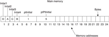
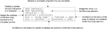
Let’s begin by declaring four char variables and initializing them with letters of the alphabet. This is shown in the first statement of the following example. The second statement declares a pointer called ptInitial and a pointer to a pointer called ptPtInitial. A pointer is declared using a signal asterisk (*). A pointer to a pointer is declared using a double asterisk (**).

char inital1 = 'D', inital2 = 'A', inital3 = 'C', inital4 = 'B';
 char *ptInitial, **ptPtInitial;
 ptInitial = &inital1;
 ptPtInitial = &ptInitial;

With variables declared, the next two statements assign values to the pointer and to the pointer to a pointer. In both cases, the ampersand (&) is used as the dereferencing operator.

The ptInitial pointer variable is assigned the address of variable inital1, which is memory address 1. The ptPtInitial pointer to a pointer variable is assigned the memory address of ptInitial. The address of ptInitial is memory address 5. Figure 2-10 shows the allocated memory after these statements execute.

Click To expand
Figure 2-10: The pointer to a pointer variable is assigned the memory address of the ptInitial pointer.

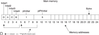
Programmers use a pointer to a pointer to tell a computer to use the contents of the memory address contained in the pointer variable that the pointer to a pointer is pointing to. This is a mouthful, so we’ll restate this using an example:

You can use the content of the inital1 variable by referencing the ptPtInitial variable. Here’s how this is done:

cout << **ptPtInitial;

The cout statement is used in C++ to display something on the screen. In this example, you’re displaying the content of the initial1 variable, although it doesn’t seem to be doing so. This statement is telling the computer to go to the memory address stored in the ptPtInitial pointer to a pointer variable, which is memory address 5 (see Figure 2-11). The content of that memory address is another memory address, which is memory address 1. The computer is told to go to memory address 1 and display the content of that memory address, which is the letter D.

Click To expand
Figure 2-11: Two memory addresses are referenced when using a pointer to a pointer to display a value on the screen.

Chapter 3: What Is an Array?

Computer memory is like a small town—or a large town, depending on the amount of memory available in the computer. Each byte of memory is a building that has its own address called a memory address, and the town’s people are bits of data living in those buildings. The small town inside your computer is a neighborly place. A program refers to buildings by name rather than by address, and puts Mary’s grade in the maryGrade building. However, being personable is troublesome when you need to come up with hundreds of names for these buildings. That is, unless you use an array. You’ll explore arrays, multidimensional arrays, pointer arrays, and an array of pointers to pointers in this chapter.

An Array

An array is a way to reference a series of memory locations using the same name. Each memory location is represented by an array element. An array element is similar to one variable except it is identified by an index value instead of a name. An index value is a number used to identify an array element.

Now we’ll show you what an array looks like, with the three array elements shown next. The array is called grades. The first array element is called grades[0]. The zero is the index value. The square bracket tells the computer that the value inside the square bracket is an index.

 grades[0]
 grades[1]
 grades[2]

Each array element is like a variable name. For example, the following variables are equivalent to array elements. There is no difference between array elements and variables—well, almost no difference, but we’ll get to the differences in a moment. For now, let’s explore how they are the same. Here are three integer variables:

 int maryGrade;
 int bobGrade;
 int amberGrade;

You probably recall from your programming class that you store a value into a memory location by using an assignment statement. Here are two assignment statements. The first assigns a value to a variable, and the other assigns a value to an array element. Notice that these statements are practically the same except reference is made to the index of the array element in the second statement:

 int grades[1];
 maryGrade = 90;
  grades[0] = 90;

Suppose you want to use the value stored in a memory location. There are a number of ways to do this in a program, but a common way is to use another assignment statement like the ones shown in the next example. The first assignment statement uses two variables, the next assignment statement uses two array elements, and the last assignment statement assigns the value referenced by a variable name and assigns that value to an array element:

 bobGrade = maryGrade;
 grades[0] = grades[1];
 grades[0] = bobGrade;

You’ve probably noticed a pattern developing. You use an array element the same way you use a variable.

Why an Array?

There are two important differences between an array element and a variable, and those differences make working with large amounts of data a breeze. Suppose you had to work with 100 grades to calculate the average grade. How would you do this?

The challenge isn’t applying the formula for calculating an average. You know how that’s done. The challenge is to come up with 100 variable names and then reference all those variable names in a program. Ouch!

First, you’d need to sum all the grades by writing a statement similar to the following. (We’ll stop at three variables because it’s difficult to identify 100 variables—and we’d run out of space on this page.)

 sum = maryGrade + bobGrade + amberGrade;

Now, here’s how a smart programmer meets this challenge using an array:

 sum = 0;
 for (int i = 0; i < 100; i++)
  sum = sum + grades[i];

Big difference. The control variable of the for loop is the index for the array element, enabling the program to quickly walk through all array elements in two lines of code. (The first statement has nothing to do with walking through all the array elements. It only initializes the sum variable with the total grades.)

The other difference between an array and a variable is that all the array elements are next to each other in memory. Variables can be anywhere in memory. For example, grades[0] is next to grades[1] in memory, grades[1] is next to grades[2] in memory, and so on. In contrast, maryGrade and bobGrade variables can be anywhere in memory, even if they are declared in the same declaration statement.

You might be scratching your head right now thinking, that’s an interesting bit of computer trivia. So what? But the location of array elements is important when pointers (see Chapter 2) are used to manipulate data stored in memory. It is more efficient to point to array elements than variables because the computer moves to the next memory location when you point to the next array element.

Arrays and Data Structures

Some programmers might say that arrays are the backbone of data structures because an array enables a programmer to easily reorganize hundreds of values stored in memory by using an array of pointers to pointers.

This is a mouthful to say. So we drew a picture to show you the importance of arrays in data structures. Figure 3-1 shows memory; you’ll remember this from the previous chapters in this book. Each block is a byte. We’ll say that two bytes are needed to store a memory address in memory. You need to store a memory address in memory because you’ll use it to refer to other memory addresses in the “An Array of Pointers” section of this chapter.

Click To expand
Figure 3-1: Elements of an array are stored sequentially in memory.

First, create an array called letters and assign characters to it, as shown here:

 char letters[3];
 letters[0] = 'C';
 letters[1] = 'B';
 letters[2] = 'A';

You’ll notice in Figure 3-1 that each letter appears one after the other in memory. This is because these values are assigned to elements of an array, and each array element is placed sequentially in memory.

Next, create an array of pointers. As you’ll recall from Chapter 2, a pointer is a variable that contains a memory address of another variable. In this example, you’ll use an array of pointers instead of a pointer variable.

An array of pointers is nearly identical to a pointer variable except each array element contains a memory address. Assign the memory address of each element of the letters array to elements of the ptLetters array, which is an array of pointers. Here’s how this is done in C and C++:

 char * ptLetters[3];
 for (int i = 0; i < 3; i++)
  ptLetters[i] = &letters[i];
 

Remember from Chapter 2 that the ampersand (&), which is called the address operator, tells the computer to assign the memory address of the element of the letters array and not the contents of the element.

The final step is to create an array of pointers to pointers and then use it to change the order of the letters array when printing the letters array on the screen. A pointer to a pointer is a variable that contains the address of another pointer. In the example, you use an array of pointers to a pointer where each element of the array is like a pointer to a pointer variable. That is, each element is assigned an address of a pointer.

Use the following code to assign the memory address of each element of the ptLetters pointer array to the ptPtLetters pointer to pointer array. Notice that you don’t use a for loop. This is because you need to change the order of the letters array without changing the letters array itself. Figure 3-1 shows how memory looks after the following code executes. If you printed elements of the ptPtLetters array, what would be displayed on the screen?

 char ** ptPTLetters[3];
 ptPtLetters[0] = &ptLetters[2];
 ptPtLetters[1] = &ptLetters[1];
 ptPtLetters[2] = &ptLetters[0];

Here is the code that prints the ptPtLetters array:

 for ( i = 0; i <3; i++)
  cout << **ptPtLetters[i] << endl;

The answer to the question is A B C. Follow Figure 3-1 as we explain how this works. The first element of the ptPtLetters array is located at memory address 10. The content of memory address 10 is 8, which is memory address 8 because memory address 10 is the last element of the array ptLetters—a pointer. The value of memory address 8 is 3, which is the memory address of the third element of the array letters.

When the computer sees the ptPtLetters[i] statement for the first time, it goes to the array element ptPtLetters[0] and reads its value, which is 8. The computer then goes to memory address 8 and reads its content because memory address 8 is a pointer. The content of memory address 8 is 3, which is the memory address of the third element of the letters array. The computer reads the content of memory address 3 and displays the content on the screen.

This can be a bit tricky to follow unless you use Figure 3-1 as a guide; you can also use Figure 3-1 to explain how the computer displays the other letters.

The importance of using arrays for data structures is that you can easily change the order of data by using pointers and pointers to pointers without having to touch the original data. Some smart programmer might tell you that you’re not saving any time or memory by using pointers and pointers to pointers to rearrange an array of characters. The programmer is correct. However, we’re juggling characters to illustrate how arrays and pointers to pointers work. In the real world, pointers typically point to a whole group of information such as a client’s name, address, phone number, and other pertinent data. Instead of juggling all that information, you need only to juggle memory addresses.

Declaring an Array

The way to declare an array depends on the programming language used to write your program. In Java, there are two techniques for declaring an array. You can declare and initialize an array either where memory is allocated at compile time or where memory is dynamically allocated at runtime. Allocation is another way of saying reserving memory.

Let’s begin by declaring an array where memory is reserved when you compile your program. This technique is similar in Java, C, and C++, except in Java you must initialize the array when the array is declared. There are four components of a statement that declares an array. These components are a data type, an array name, the total number of array element to create, and a semicolon (;). The semicolon tells the computer that the preceding is a statement. Here’s the declaration statement in C and C++:

 int grades[10];

In Java, you must initialize the array when the array is declared as shown here. The size of the array is automatically determined by counting the number of values within the braces. Therefore, there isn’t any need to place the size of the array within the square brackets:

 int[] grades = {0,0,0,0,0,0,0,0,0,0};

The data type is a keyword that tells the computer the amount of memory to reserve for each element of the array. In this example, the computer is told to reserve enough memory to store an integer for each array element.

The array name is the name you use within a program to reference an array element. The array name in this example is grades. The number within the square brackets is the total number of elements that will be in the array. The previous statements tell the computer to create an array of 10 elements.

Avoid making a common rookie mistake. Previously in this chapter you learned that the index for the first array element is zero, not one. Therefore, the tenth array element has the index value 9, not 10.

Some programs confuse an index with the total number of array elements. That is, they use the value 9 within the square brackets when declaring an array because they assume they are declaring 10 elements. In reality, they are declaring an array of 9 elements. The confusion stems from the fact that 9 is the index to reference the tenth array element.

With a little practice you can avoid making this mistake. Remember that the value within the square brackets in the statement that creates an array is not an index, although it resembles an index. This value is the number of array elements you need. That is, you insert the number 10 within the square brackets if you need 10 array elements. You use the index value of 9 if you want to access the tenth element.

In order to allocate memory at compile time, you must know the number of array elements that you need. Sometimes you don’t know this, especially if your program loads the array with data stored in a database. The amount of data stored in a database typically fluctuates.

The solution in Java is to allocate memory at runtime. Programmers call this dynamically allocating memory. You dynamically allocate memory by using the new operator when declaring the array, as shown here:

 int grades[] = new int[10];

This example looks a little strange, but it creates the same array as is created in the previous example. There are three things happening in this statement.

First, the new operator tells the computer to reserve 10 array elements, each the size of an int data type. The new operator returns a reference to the allocated memory.

Next, a reference to an int data type called grades is declared (int grades[]).

Last, the reference to the memory allocation returned by the new operator is assigned to the reference declared in the program.

This can be confusing even for experienced programmers to understand. If you’re confused, remember this visitor’s locker room example: a stadium has a locker room with “Visitors” on the door. This is similar to the reference grades[]. The visitor’s locker room refers to the visiting team similar to the way grades[] refers to allocated memory: each game brings in a different visiting team who is assigned to the visitor’s locker room. This is similar to assigning allocated memory to the reference grades[].

Multidimensional Arrays

The array described in this chapter is referred to as a one-dimensional array because the array consists of one series of elements. However, an array can have more than one series of elements. This is called a multidimensional array.

A multidimensional array consists of two or more arrays defined by sets of array elements, as shown in Figure 3-2. Each set of array elements is an array. The first set of array elements is considered the primary array, and the second and subsequent sets of array elements are considered subarrays.


Figure 3-2: A two-dimensional array is a multidimensional array consisting of two arrays.

There are two arrays in the multidimensional array shown in Figure 3-2. Each element of the first array points to a corresponding array. For example, letters[1] in Figure 3-2 points to the array beginning with array element letters[1][0] where the zero is the first element of the second array.

Although you can create an array with any size multidimension, many programmers limit an array to two dimensions. Any size greater than two dimensions becomes unwieldy to manage.

An analogy we find helpful is visualizing a table (rows and columns) for a two-dimensional array and a cube (or similar figure) for a three-dimensional array.

Why Use a Multidimensional Array?

A multidimensional array can be useful to organize subgroups of data within an array. Let’s say that a student has three grades, a mid-term grade, a final exam grade, and a final grade. You can store all three grades for an endless number of students in a two-dimensional array, as shown in Figure 3-3.

Click To expand
Figure 3-3: All three grades can be stored in a multidimensional array.

Figure 3-3 declares a multidimensional array of integers. The first set of array elements contains three array elements, one for each student. The second set of array elements has four array elements. The first of the four elements contains the student ID and the other three contain the three grades for that student ID.

In addition to organizing data stored in elements of an array, a multidimensional array can store memory addresses of data in a pointer array and an array of pointers to pointers, which are discussed later in “An Array of Pointers to Pointers.”

Multidimensional Array in Memory

Data stored in a multidimensional array is stored sequentially by sets of elements, as shown in Figure 3-4. The first set of four array elements is placed in memory, followed by the second set of four array elements, and so on.

Click To expand
Figure 3-4: Elements of a multidimensional array are stored sequentially in memory.

The name of a multidimensional array references the memory address of the first element of the first set of four elements. That is, grades is the equivalent of using memory address 1 in Figure 3-4. You can use the name of a multidimensional array as a pointer to the entire array.

The index of the first element of the first set of array elements points to the memory address where values assigned to array elements are stored.

Referencing the index of the first dimension points to the memory address of the first element of that dimension. For example, referencing grades[1] points to memory address 9 in Figure 3-4. Memory address 9 is the first memory address of contiguous memory where values of the second set of array elements that are associated with grades[1] are stored.

Declaring a Multidimensional Array

A multidimensional array is declared similar to the way you declare a one-dimensional array except you specify the number of elements in both dimensions. For example, the multidimensional array shown in Figure 3-3 is declared as follows in C or C++:

 int grades[3][4];

The first bracket ([3]) tells the compiler that you’re declaring 3 pointers, each pointing to an array. This concept might be confusing because the term “pointer” may make some programmers think of pointer variable or pointer array, which you’ll learn about later in this chapter. However, we are not talking about a pointer variable or pointer array. Instead, we are saying that each element of the first dimension of a multidimensional array reference a corresponding second dimension, which is an array.

In this example, all the arrays pointed to by the first index are of the same size. The second index can be of variable size. For example, the previous statement declares a two-dimensional array where there are 3 elements in the first dimension and 4 elements in the second dimension.

The element grades[0] is said to “point” (just as you use your finger to point) to the second dimension of the array, which is referenced as grades[0][0]. The second dimension is considered an array. Therefore, programmers say that the first element of a multidimensional array points to another array (that is, the second dimension).

The data type tells the computer that each element of the array will contain an integer data type. The data type is followed by the array name and two values that indicate the size of each dimension used for the array. In this case, there are three sets of four array elements.

You declare a multidimensional array and initialize its elements by using French braces, as shown in Figure 3-5. There are three sets of inner French braces. Each of these sets represents the first dimension of the array. There are four values within each set of inner French braces. These values are assigned to each element of the second dimension of the array.

Click To expand
Figure 3-5: Braces define sets of values to be assigned to array elements (the top example is C and C++ and the bottom example is Java).

Assigning Values to a Multidimensional Array

You assign a value to an element of a multidimensional array with an assignment statement similar to the assignment statement that assigns a value to a single-dimensional array, as shown here:

 grades[0][0] = 1001;

You must specify the index for both dimensions. In this example, the integer 1001, which is a student ID, is assigned to the first element of the first set of elements in the grades array.

Referencing the Contents of aMultidimensionalArray

The contents of elements of a multidimensional array can be used in a program by referencing the index of both dimensions of the array element. Figure 3-6 shows you how to display the final exam grade for the second student.

Click To expand
Figure 3-6: Display the contents of array elements by referencing the index of both sets of array elements.

In this example, the student ID is displayed by referencing the first element of the second set, and the grade for the final exam is displayed by referencing the third element of the second set.

Pointers and Arrays

There is a close-knit relationship between a pointer and an array. The array name is like a pointer variable in that the array name by itself references the address of the first element of the array. Confused? We’ll give you an example (see Figure 3-7) to show how this works.

Click To expand
Figure 3-7: Use the array name as a pointer to the first array element.

Java doesn’t permit a programmer to use pointers, so we use C++ code in Figure 3-7. The example begins by declaring an array of characters called letters that consists of 2 elements. Also declared is a character pointer called ptLetters. (You learned about pointers in Chapter 2.)

Next, the character A is assigned to the first element of the array. The address of the first array element is then assigned to the pointer variable. Figure 3-8 gives you a glimpse of memory once the address of the first array element is assigned to the pointer.

Click To expand
Figure 3-8: Memory allocation after the pointer is assigned the address of the first array element

Figure 3-7 displays the letter A twice. The first time is by using the name of the array as a pointer. Only the name of the array is used—the square brackets and index are not. The A is displayed the second time by using the pointer. Using the asterisk dereferences both the array name and the pointer. (You learned about dereferencing in Chapter 2.)

You might be wondering why you’d use the array name as a pointer to the first element of the array. Programmers do this to use pointer arithmetic (see the “Pointer Arithmetic” section of Chapter 2) to access each array element without having to reference an array index.

An Array of Pointers

Previously, you learned that pointers are the backbone of data structures. Some programmers feel that an array of pointers, also known as a pointer array, is the backbone of pointers. An array of pointers is an array whose elements are pointers. That is, the value of each array element is a memory address similar to a pointer variable, which you learned about in Chapter 2.

The benefit of using an array of pointers instead of several pointer variables is that you can use a for loop to step through each element of the array to access memory addresses that are assigned to the array. You’ll need to do this to efficiently access and reorder values stored in memory.

An array of pointers is not available in all programming languages. For example, Java doesn’t let programmers use pointers, so you won’t be able to create an array of pointers in Java. However, you can create an array of pointers in C and C++.

Note

It is technically incorrect to say that Java doesn’t use pointers. Java does use pointers, but a programmer doesn’t explicitly declare them. You can declare an array whose data type is a Java object, and this is in fact an array of pointers. The value of each array element is an object. When you switch those values to other array elements, you are moving memory addresses and not the object itself.

An array of pointers is declared using nearly the same format as declaring an array of data types, with one exception. The name of the array must be preceded with an asterisk, as shown here:

 char *grades[10];

The asterisk tells the computer that the array is a pointer array where each element can contain a memory address. The data type in this declaration statement tells the computer that memory addresses stored in array elements are memory addresses that contain a char value. This is the same pointer variable concept you learned in Chapter 2.

As you probably recall from your programming course, a computer copies the value of a variable in an assignment statement, as shown in the next example. The first two statements in this example reserve a memory location large enough to store a char and associate those memory addresses with the names finalGrade and recordedGrade. The first statement also stores the value A in memory. The last statement copies the value stored in the memory location represented by finalGrade to the memory address represented by the recordedGrade.

 char finalGrade = 'A';
 char recordedGrade;
 recordedGrade = finalGrade;

You assign a memory address of a variable to an element of an array of pointers by placing the address operator (&) in front of a variable name in an assignment statement to reference the variable. The ampersand (&) returns a pointer, and an asterisk (*) dereferences the pointer and tells the computer that you want the value pointed to by the pointer.

Referencing tells the computer to copy the memory address of the variable instead of copying the value stored in the memory address. This is illustrated in the next example where the address of the finalGrade variable is referenced, resulting in the memory address of the finalGrade variable being assigned to the first element of the ptRecordedGrades array. The ptRecordedGrades is an array of pointers.

 char finalGrade = 'A';
 char *ptRecordedGrades[10];
 ptRecordedGrades[0] = &finalGrade;

Programmers use an array of pointers in two ways: they use the address assigned to array elements, and they use the content of the memory address assigned to an array element. Let’s take a look at how to use addresses stored in an array of pointers.

The following example initializes three variables with grades and declares two pointer arrays called ptGradeBook and ptRecordedGrade. The addresses of the three variables are then assigned to each element of the ptGradeBook pointer array. A for loop then copies memory addresses stored in the ptGradeBook array to the ptRecordedGrade array. Notice that the ampersand is not used in this assignment expression because we want the content of each array element to be copied to the ptRecordedGrade array.

 char bobGrade = 'A';
 char maryGrade = 'B';
 char amberGrade = 'A';
 char *ptGradeBook[3];
 char *ptRecordedGrade[3];
 ptGradeBook [0] = &bobGrade;
 ptGradeBook [1] = &maryGrade;
 ptGradeBook [2] = &amberGrade;
 for (int i = 0; i < 3; i++)
  ptRecordedGrade[i] = ptGradeBook[i];

Now we’ll modify this program slightly in the next example by changing the ptRecordedGrade array from an array of pointers to an array of integers. We’ll then use the for loop to copy the contents of the variables to the recordedGrade by using the pointer array, as shown here:

 char bobGrade = 'A';
 char maryGrade = 'B';
 char amberGrade = 'A';
 char *ptGradeBook[3];
 char recordedGrade[3];
 ptGradeBook [0] = &bobGrade;
 ptGradeBook [1] = &maryGrade;
 ptGradeBook [2] = &amberGrade;
 for (int i = 0; i < 3; i++)
  recordedGrade[i] = *ptGradeBook[i];

The last statement in this example dereferences each element of the ptGradeBook array by preceding the name of the array with an asterisk. This tells the computer to first go to the memory address stored in the array element and then copy the value stored at the memory address to the element of the recordedGrade array element (see Figure 3-9).

An Array of Pointers to Pointers

The supercharger of pointers is an array of pointers to pointers because an array of pointers to pointers enables you to reorganize tons of data in memory by simply referring to memory addresses. You were introduced to arrays of pointers to pointers at the beginning of this chapter. You’ll now learn the ins and outs of using them.

Be forewarned: an array of pointers to pointers is one of the most abstract concepts to grasp in programming. Therefore, it is critical that you draw a picture of computer memory as you analyze a program that uses an array of pointers to pointers; otherwise, you are bound to become unnecessarily frustrated.

Let’s begin by recalling the basics. It probably seems that you read these terms countless times in the last chapter and this chapter, but these terms are so important to understanding an array of pointers to pointers that we’ll talk about them one more time.

A variable is a reference to a memory location used to store data that is described in a data type. A pointer variable is the same as a variable except its contents are the memory address of another variable. A pointer to a pointer, which you learned about in Chapter 2, is a pointer variable. The contents of the pointer variable is a memory address of another pointer variable.

More on an Array of Pointers to Pointers

Before we show you how to use an array of pointers to pointers, let’s be sure that you understand how arrays, arrays of pointers, and arrays of pointers to pointers join forces to rearrange tons of data efficiently.

Think of an array as the storage place of the tons of data. The last thing you want to do is to physically reorganize a lot of data in computer memory because it is inefficient.

Think of an array of pointers as the storage place for memory addresses of data stored in an array. This is like a notepad where you jot down memory addresses of data.

Think of an array of pointers to pointers as the place where you reorganize the data contained in the array by indirectly rearranging memory addresses contained in the array of pointers. You can have any number of arrays of pointers to pointers, each indirectly ordering the content of the array of pointers in a different order.

Let’s say that you have a list of three names, as shown in Figure 3-10. Each name is assigned to elements of an array in reverse alphabetical order. You can reorder those names without changing their order in the array by using an array of pointers and an array of pointers to pointers.

Click To expand
Figure 3-10: An array of pointers to pointers reorganizes names without changing the order of the array that contains the names.

In Figure 3-10, elements of the array of pointers are assigned the memory addresses of each element of the array. Elements of the array of pointers to pointers are assigned the memory addresses of elements of the array of pointers. Notice that these memory addresses are assigned in the reverse order that they appear in the array of pointers, which indirectly references the array of names in reverse order—that is, in alphabetical order.

Declaring and Using an Array of Pointers to Pointers

An array of pointers to pointers is declared nearly the same way as you declare an array of pointers, except two asterisks (**) are used before the name of the array, as shown here:

 string **ptPTStudents[3];

The data type of an array of pointers to pointers is used a little differently than the data type of an array of pointers. Previously in this chapter, you learned that the data type of an array of pointers refers to the data type stored at memory addresses that are assigned to elements of the pointer array.

Suppose you declared an array of strings and an array of pointers to strings and then assigned memory addresses of the string array to the pointer array. The data type of the pointer array is a string data type, which tells the computer that elements of the pointer array contain memory addresses of strings.

The data type of the array of pointers to pointers corresponds to the data type of the pointers that are assigned to elements of the array of pointers to pointers. Let’s say you assign elements of the pointer array to elements of the array of pointers to pointers. Because the pointer array points to strings, the array of pointers to pointers must also use the string data type.

The data type of an array of pointers to pointers tells the computer that the memory address contains a memory address that is a pointer. This pointer contains a memory address of a string or whatever the data type specified when the pointer is declared.

Assigning Values to Elements of anArrayofPointerstoPointers

You assign a value to an element of an array of pointers to pointers the same way you assign a value to an element of an array of pointers. That is, use the address operator (&) to reference either a pointer variable or an element of an array of pointers, as shown here:

 ptPTStudents[0] = &ptStudents[0];

You’ll recall that the address operator tells the computer to assign the memory address of a pointer variable or array element to the element of the array of pointers to pointers, not the value stored at that address. The previous example assigns the memory address of a pointer array to the element of the array of pointers to pointers. It does not assign the contents of the ptStudents[0], which is also a memory address.

Using the Contents of an Array of Pointers to Pointers

Accessing the contents of an element of an array of pointers to pointers is nearly identical to the way the content of an element of a pointer array is accessed. Previously, you learned that you dereference an element of a pointer array when you want to tell the computer to use the content of the element, as shown here:

 cout << *ptStudents[0] << endl;

An element of an array of pointers to pointers is accessed by using two asterisks (**), as shown in this statement:

 cout << **ptPTStudents[0] << endl;

Pointers to Pointers in Action

Now that you have a firm grasp on arrays and an array of pointers to pointers, we’ll show you how you can harness the power of the array. Figure 3-10 is a diagram of how an array containing three names is reordered using a pointer array and an array of pointers to pointers. Figure 3-11 shows how to do this in C and C++. Remember that Java does not permit programmers to use pointers directly, but understanding how pointers work in C and C++ will help you understand how pointers are used in Java.

Click To expand
Figure 3-11: Using a pointer array and an array of pointers to pointers to display the contents of an array of strings

The program begins by declaring an array of strings called students that is initialized with the names of three students. Notice the order of these names. The program will use an array of pointers to pointers to reverse this order.

Once the array of strings is declared, the program declares a pointer array and an array of pointers to pointers, both of which have three elements. Two integers are then declared and used as control variables for the for loop.

The first for loop displays elements of the students array to show the original order in which names are stored in the array, as shown in the left stack in Figure 3-10.

The second for loop assigns memory addresses of each element of the students array to elements of the pointer array, as shown in the center stack in Figure 3-10.

The third for loop uses the ptStudents array of pointers to display students contained in the students array. Names appear in the same order shown in the left stack in Figure 3-10.

The fourth for loop assigns the memory address of each element in the pointer array to elements of the array of pointers to pointers, which is called ptPtStudents. This is where the program reorders names of the students array. It may look confusing at first glance, but here’s what is happening.

The i control variable is initialized to 0, and the x control variable is initialized to 2. These determine the starting points in the array of pointers to pointers and the pointer array. The ptPtStudents pointer to pointer array begins with the first element, while the ptStudents array pointer begins with the last element. This is because the program reverses the order in which names appear in the students array. The last name will appear first in the reordered list.

Each time the for loop is looped, the value of the i variable is incremented, causing the program to move to the second and third elements of the ptPtStudents array of pointers to pointers. At the same time, the value of the x variable is decremented, causing the ptStudents pointer array to move to the second and first elements, as shown in the right stack in Figure 3-10.

The fifth for loop steps through elements of the ptPtStudents array of pointers to pointers displaying the corresponding name in the students array on the screen.

Chapter 4: Stacks Using anArray

The term “stack” is one of the magical and sometimes imposing terms used in computer programming that seems to imply an abstract concept that only a Ph.D. from MIT—whoops, we should say Columbia University—can understand. Yet you actually know all about stacks because you use a stack when playing cards, making pancakes, and storing laundry. A stack is the way you groups things together by placing one thing on top of another and then removing things one at a time from the top of the stack. It is amazing that something this simple is a critical component of nearly every program that is written. In this chapter, you’ll learn how to create and use a stack in your programs.

A Stack

When you hear the term “stack” used outside the context of computer programming, you might envision a stack of dishes on your kitchen counter. This organization is structured in a particular way: the newest dish is on top and the oldest is on the bottom of the stack.

Each dish in a stack is accessed using fifo: first in, first out. The only way to access each dish is from the top of the stack. If you want the third dish (the third oldest on the stack), then you must remove the first two dishes from the top of the stack. This places the third dish at the top of the stack making it available to be removed.

There’s no way to access a dish unless the dish is at the top of the stack. You might be thinking stacks are inefficient, and you’d be correct if the objective was to randomly access things on the stack. There are other data structures that are ideal for random access, which you’ll learn about throughout this book.

However, if the object is to access things in the order in which they were placed on the stack, such as computer instructions, stacks are efficient. In these situations, using a stack makes a lot of sense.

Note

Stacks and arrays are often bantered about in the same discussion, which can easily lead to confusion, but they are really two separate things (see Figure 4-1). An array stores values in memory; a stack tracks which array element is at the top of the stack. When a value is popped off the stack, the value remains in memory because the value is still assigned to an array element. Popping it only changes the array element that is at the top of the stack.

Click To expand
Figure 4-1: A stack and an array are two different things: an array stores values in memory; a stack tracks which of the array elements is at the top of the stack.

Inside a Stack

Programmers use arrays to store values that are referenced by a stack. As you’ll recall from Chapter 3, an array consists of a series of array elements, each of which is similar in concept to a variable. The stack contains the index of the array element that is at the top of the stack.

Figure 4-1 is the way some programmers envision an array used with a stack. This example shows an array called stack with 8 array elements. The entire array contains values that are referenced by the stack. Three array elements are assigned values, while the other array elements are empty and can be used when new items are placed on the stack (see the upcoming section “Push”).

Mike is the first value placed on the stack. You know this because Mike is at the bottom of the stack. Bob is the last item placed on the stack because Bob is the top item on the stack.

Push

Programmers use the term “push” to mean placing an item on a stack. Push is the direction that data is being added to the stack. Think of this as pushing items down on the stack to move the items already on the stack down to make room for the next item.

Here’s what actually happens. The new value is assigned to the next available array element and the index of that array element becomes the top of the stack, as shown in Figure 4-2. The program increments the current index of the stack by 1. In this example, the index is incremented by 1, resulting in index 3 being at the top of the stack, which is the index of the new values assigned to the array.

Click To expand
Figure 4-2: The new value is assigned to the next array element and its index becomes the top of the stack.

Pop

Popping is the reverse process of pushing: it removes an item from the stack. It is important to understand that popping an item off the stack doesn’t copy the item. Once an item is popped from the stack, the item is no longer available on the stack, although the value remains in the array.

Here’s what really happens. Remember that the top of the stack contains an index of the array element whose value is at the top of the stack. In Figure 4-2, index 3 is at the top of the stack, which means New Value in array element 3 is at the top of the stack.

When you pop New Value from the stack, you decrement the index at the top of the stack. That is, you make its index 2 instead of 3. This makes Bob the new value at the top of the stack (see Figure 4-3). Notice that New Value and array element 3 remain untouched in the array because popping a value from the stack only alters the stack, not the underlying array.

Click To expand
Figure 4-3: All values move toward the top of the stack when the top item is popped off the stack.

Creating a Stack in C++

You can create a stack in C++ by defining a stack class and declaring an instance of the class. The Stack class requires three attributes and several member functions, which are defined as you learn about them. You’ll begin by defining a basic stack class that has only the components needed to create the stack.

The class is called Stack, but you can call it any name you wish. This class definition is divided into a private access specifier section and a public access specifier section. The private access specifier section has attributes and member functions (although not in this example) that are accessible only by a member function defined in this class. The public access specifier section has attributes (although not in this example) and member functions that are accessible by using an instance of the class.

The private access specifier section of the Stack class defines three attributes: size, top, and values, all of which are integers. The size attribute stores the number of elements in the stack, the top attribute stores the index of the top element of the stack, and the values attribute is a pointer to the stack, which is an array. The stack in this example is a stack of integer values, but you can use an array of any data type, depending on the nature of your program.

Only one member function is defined in the Stack class, although we’ll define other member functions for the class in upcoming sections of this chapter. For now, let’s keep the example simple and easy to understand.

This member function is called Stack, which is the constructor of the class. A constructor is a member function that has the same name as the class and is called when an instance of the class is created. The code for this is on the next page.

Several things are happening in the constructor. First, the constructor receives an integer as an argument that is passed when the instance of the Stack class is declared. The integer determines the number of elements in the stack and is assigned to the size variable.

The first statement might look a bit confusing. It appears that the value of the size variable from the argument list is being assigned to itself, but that’s not the case. Actually, the size variable from the argument list is local to the Stack member function. The this->size combination refers to the size attribute of the Stack class, as shown here:

this->size = size;

Programmers use the this pointer within a member function to refer to the current instance of the class. In this example, the this pointer uses the pointer reference (->) to tell the computer to use the size attribute of the class. As you’ll remember from your C++ programming class, the pointer reference is used when indirectly working with a class member, and the dot operator is used when you are directly working with a class member.

This allows the compiler to distinguish between a class variable and local variable that have the same name. This means that the value of the size variable that is passed as an argument to the Stack member function is assigned to the size attribute, making the value available to other members of the Stack class.

You can see how the size attribute is used in the next statement. This statement does two things. First, it allocates memory for the stack by using the new operator (new int[size]). The new operator returns a pointer to the reserved memory location. The size is the size attribute of the class and determines the size of the array. The array is an array of integers.

Next, the pointer to the array of integers is assigned to the values attribute of the class. The values attribute is a pointer variable that is defined in the private attribute section of the Stack class.

The last statement in the Stack member function assigns a –1 to the top attribute. The value of the top attribute is the index of the top element of the stack. A –1 means that that stack doesn’t have any elements. Remember from your programming class that index values are memory offsets from the start of the array. Index 0 means “move 0 bytes from the start of the array.” So index –1 is just a convenient way to say that the stack is empty.

We’ll expand on the definition of the Stack class in the next section, but for now let’s create an instance of the Stack class. The instance is declared within the main() function of this example. Three things are happening here. First, the new operator is creating an instance of the stack in memory. The new operator returns a pointer to that memory location.

Next, the statement declares a reference to the stack, which is called myStack. The reference is a pointer. The final step is to assign the pointer returned by the new operator to the reference. You then use the reference (myStack) as the name of the instance of the Stack class throughout the program.

public class Stack
 {
  private:
  int size;
  int top;
  int* values;
  public:
  Stack(int size)
  {
  this->size = size;
  values = new int[size];
  top = -1;
  }
 };
 void main(){
  Stack *myStack = new Stack(10);
 }

Creating a Push Member Function in C++

Now that you’ve seen how to define a class that creates a stack, we’ll show you how to define additional member functions that enable the class to push values onto the stack. Pushing a value onto the stack is a two-step process. First, you must determine if there is room on the stack for another value. If there is, you push the value onto the stack; otherwise, you don’t.

We’ll create different member functions for each step, beginning by defining a member function that determines if there is room on the stack. We’ll call it isFull() and define it in the following code. The isFull() member function is simple. It compares the value of the top attribute with the one less than the value of the size attribute.

The value of the top attribute is –1 when the instance of the stack is declared. Suppose the value of size is 10. The condition expression in the if statement of the isFull() member function determines if the value of top, which is –1, is 1 less than the value of size. Since the value of size is 10, the condition expression compares –1 < 9. If top is greater than or equal to 9, then a true is returned; otherwise, a false is returned.

Why do you subtract 1 from the size of the stack? The value of the top attribute is an index of an array element. Remember that the index begins with zero. In contrast, the size is actually the number of array elements in the stack. Therefore, the tenth array element on the stack has an index of 9.

bool isFull()
 {
  if(top < size-1)
  {
  return false;
  }
  else
  {
  return true;
  }
 }

With the isFull() member function defined, we’ll move on to defining the push() member function, as shown in the next example. The push() member function pushes a value onto the stack. The value being pushed onto the stack is passed as an argument to the push() member function and is assigned to the variable x in this example.

Before doing anything else, the push() member function determines if there is room on the stack by calling the isFull() member function in the condition expression of the if statement. The condition expression might look a little strange because the call is preceded by an exclamation point (!) so we’ll take apart the condition expression to explain what is really happening here.

Remember from your programming classes that statements within an if statement execute only if the condition expression is true. This means the condition expression must be true for the value passed to the push() member function to be placed on the stack.

Here’s a slight problem. We’re calling the isFull() member function to determine if there is room on the stack for another value. However, the isFull() member function returns false if there is room and true if there isn’t room. A false causes the push() member function to skip statements that place the value on the stack. We really need the isFull() member function to return a true if there is room available, not a false. Rather than rewrite the isFull() member function, we use the exclamation point to reverse the logic. As you remember from your programming class, the exclamation point is the not operator—that is, a false is treated as a true, which causes the value to be placed on the stack.

There are two statements within the if statement. The first statement increments the value of the top attribute, which is the index of the last value placed on the stack. If the stack is empty, then the current value of the top attribute is –1. Incrementing –1 changes the value of the top attribute to 0, which is the index of the first array element of the stack. The last statement in the if statement assigns the value passed to the push() member function to the next available array element.

void push(int x)
 {
  if(!isFull())
  {
  top++;
  values[top] = x;
  }
 }

Creating a Pop Member Function in C++

We still need a way to remove values from the stack. To do this, we need to define two additional member functions, isEmpty() and pop(). The isEmpty() member function determines if there are any values on the stack. The pop() member function removes the value from the top of the stack.

Let’s define the isEmpty() member function in this next example. The isEmpty() member function contains an if statement. The condition expression of the if statement compares the value of the top attribute to –1. Remember that –1 is the initial value of the top attribute when the instance of a stack is declared. If the top attribute is equal to –1, then a true is returned because the stack is empty; otherwise, a false is returned.

bool isEmpty()
 {
  if(top == -1)
  {
  return true;
  }
  else
  {
  return false;
  }
 }

The pop() member function of the Stack class has the job of changing the index that is at the top of the stack and returning the value of the corresponding array to the statement that calls the pop() member function. The next example defines the pop() member function.

The first statement in the definition declares an integer variable called retVal that stores the value returned by the pop() member function. The retVal is initialized to zero.

Next, the isEmpty() member function is called in the condition expression of the if statement to determine if there is a value at the top of the stack. Notice the exclamation point reverses the logic as it did in the pop() member function.

Statements within the if statement should only execute if the isEmpty() member function returns a false, meaning the stack is not empty. Therefore, we need to use the exclamation point to reverse the logic of the condition expression to make the condition expression true if the isEmpty() member function returns a false.

Two steps occur within the if statement. First, the value at the top of the stack is assigned to the retVal variable by referencing the values array using the index contained in the top attribute. Next, the value of the top attribute is decremented. The return retVal is then returned by the pop() member function.

int pop()
 {
  int retVal = 0;
  if(!isEmpty())
  {
  retVal = values[top];
  top--;
  }
  return retVal;
 }

Stack in Action Using C++

Now that you understand how to create and use a stack, we’ll pick up the pace and explore an industrial-strength stack. You’ve may have heard the term industrial strength used in relation to programming and may be curious what this really means.

Industrial strength is a term used in industry that implies a product is designed to withstand stress. Industrial strength can be used to describe any kind of product, but in this case the product is the program that creates and uses a stack.

Programs used to illustrate the concepts of a stack in this chapter are bare bones and lack the robust features that are found in industrial-strength programs. A bare-bones program is what you need when you’re learning the concepts of stacks and other data structures because the program contains only statements that pertain to what you are learning.

However, once you learn the concept, you need to see how it’s applied in a real-world program. That’s what we’ll be exploring in the “Stack in Action” sections of this chapter. In this section, you’ll take a look at how a stack is created and used in an industrial-strength C++ program. Later, you’ll see the Java version of this program.

Tip

From your programming classes, you learned to always build error-trapping routines into your program to properly handle errors should they occur. Always include such routines in your stack program. Three common errors to trap are problems allocating memory for the stack, reacting to a full stack, and reacting to an empty stack.

We’ll use as an example an industrial-strength C++ program that creates and uses a stack. The program is contained within three files, stack.h, stack.cpp, and stackDemo.cpp. The stack.h file is a header file that contains the definition of the Stack class, which is the “blueprint” of the Stack class. The stack.cpp file is a source code file that contains the implementation of the member functions of the Stack class. The stackDemo.cpp file contains the source code for the C++ program that declares the instance of the Stack class and calls its member functions. Let’s begin by taking a look at the stack.h header file, which is shown in the next code example. As you’ll recall from your C++ classes, a header file typically contains definitions and preprocessor instructions. A preprocessor is a program that applies preprocessor instructions to source code before the code is compiled.

The stack.h header file contains one preprocessor instruction, #define, which defines a symbol. Here we’ve defined the symbol DEFAULT_SIZE and given it a value of 10. The preprocessor then replaces all occurrences of DEFAULT_SIZE with 10 before the code is compiled. The DEFAULT_SIZE is the default size of the stack if the no argument is passed to the constructor. Function parameters in C and C++ can be assigned default values in the function prototype as long as those arguments are at the end of the argument list. If the size value is not passed in, it gets defaulted to the value of DEFAULT_SIZE, which is 10 in our example.

The stack.h file also contains the definition of the Stack class. The Stack class definition has the same size, top, and values attributes you saw in the previous C++ example. However, the definition of member functions is different from what you saw because member functions are implemented outside the class definition in the stack.cpp source code file. The header file contains only the prototype of the functions, which make up the blueprint for the class.

From your C++ class, you’ll remember that only the prototype or signature of a member function needs to be included in a class definition. The implementation of the member function can be outside the class definition. There are two important reasons for keeping the definition (header file) and implementation (source) in separate files:

  • It keeps your development environment cleaner and easier to understand.

  • It allows you to provide a commercial software application programmer interface to a programmer without handing over your source code. You provide the programmer with your header files, which they will use to compile their code (they only need header files to compile the code). You provide your source code in the form of precompiled libraries that are referenced by the programmer’s program during linking.

The class definition contains signatures of six member functions. The first member function is called Stack, which is the constructor that you learned about previously in this chapter. Previously, you learned that the constructor is passed an integer representing the size of the stack. In the real-world version, the program sets a default size that can be overridden when an instance of the class is created in the program. The default size is specified by using the DEFAULT_SIZE, which is 10 (see #define).

The next member function is ~Stack() and is the destructor of the class. A destructor is the last member function that is called when the instance of the class goes out of scope and dies. A constructor must always be the same name as the class and begin with a tilde (~). By definition, destructors cannot accept any arguments. The purpose of the destructor is to free memory that is used by the stack or do any other sort of cleanup that’s required.

The remaining member functions are the same functions that you learned about previously in this chapter.

//stack.h
 #define DEFAULT_SIZE 10
 class Stack 
 {
  private:
  int size;
  int top;
  int* values;
  public:
  Stack(int size = DEFAULT_SIZE);
  virtual ~Stack();
  bool isFull();
  bool isEmpty();
  void push(int);
  int pop();
 };
 

The stack.cpp file is a source code file that contains the implementation of the Stack class’s member functions. We placed these in a different file from the class definition because it is easier to read and maintain as well as for other reasons explained previously.

The file begins with the preprocessor instruction #include that tells the computer to evaluate the contents of the stack.h file before compiling the stack.cpp file so it “knows” about the Stack class definition before compiling the program.

Member functions in the stack.cpp file will be familiar to you because all except one are the same member functions that you learned about previously in the chapter. However, the names of the member functions might be confusing at first glance because each name begins with the name of the class followed by two colons (::). The two colons are called the scope resolution operator.

You must precede the name of a member function with the class name and scope resolution operator if the member function is defined outside the class definition. Think of this as telling the computer that the member function belongs to the Stack class.

The ~Stack() member function frees memory used by the stack. It does this by using the delete operator and referencing the name of the array used for the stack. In this example, values is the name of the array.

To avoid memory leaks, freeing memory is important whenever memory is dynamically allocated. The square brackets ([]) are used with delete because the object being removed from memory was dynamically created.

The stack.cpp is compiled as you would compile any source code. The result is an object file that is joined together with the compiled stackDemo.cpp source code file by the linker to create an executable program called a load module.

//stack.cpp
 #include "stack.h"
 Stack::Stack(int size)
 {
  this->size = size;
  values = new int[size];
  top = -1;
 }
 Stack::~Stack()
 {
  delete[] values;
 }
 bool Stack::isFull()
 {
  if(top < size-1)
  {
  return false;
  }
  else
  {
  return true;
  }
 }
 bool Stack::isEmpty()
 {
  if(top == -1)
  {
  return true;
  }
  else
  {
  return false;
  }
 }
 void Stack::push(int x)
 {
  if(!isFull())
  {
  top++;
  values[top] = x;
  }
 }
 int Stack::pop()
 {
  int retVal = 0;
  if(!isEmpty())
  {
  retVal = values[top];
  top--;
  }    
  return retVal;
 }

Finally, we come to the stackDemo.cpp program, which is the C++ program that creates the instance of the Stack class. The first statement creates the stack in a three-step process. The first step is to use the new operator to allocate space in memory for the Stack class by calling the constructor of the class. The new operator returns the memory location of the stack. The second step is to declare a pointer called stack. The last step is to assign the memory location returned by the new operator to the stack pointer.

In this example, we used the default size for the stack, which is 10 elements. We can pass the Stack() constructor an integer to change the size of the stack.

The push() member function is called three times. Each time a different value is placed on the stack. Notice that the -> pointer is used instead of the dot operator. You must do this because stack is a pointer to an instance of the class and not the instance itself.

The last portion of the stackDemo.cpp program calls the pop() member three times. Each time a value is removed from the top of the stack and displayed on the screen.

//stackDemo.cpp
 void main() {
  Stack *stack = new Stack();
  stack->push(10);
  stack->push(20);
  stack->push(30);
  for(int i=0; i<3; i++)
  {
  cout << stack->pop() << endl;
  }
 }

Chapter 5: Queues Using anArray

You probably never thought that waiting in line in the supermarket would help you become a whiz at data structures, but it’s a big help: the checkout line at a supermarket is similar to the way data structures are organized. We’re the “things” organized by the supermarket line, and the same kind of organization is used for data within your program. The checkout line in your program is called a queue. In this chapter, you’ll learn the ins and outs of implementing a queue within your program.

A Queue

A queue is like the checkout line at the supermarket where the first customer is at the front of the line, the second customer is next in line, and so on until you reach the last customer who is at the back of the line. Customers check out of the supermarket in the order they arrive in the line. That is, the first customer is the first one to check out. This is referred to as first in, first out (fifo).

The same concept applies to a queue in your program. A queue is a sequential organization of data. Data is accessible using fifo. That is, the first data in the queue is the first data that is accessible by your program. In this chapter, you will explore the simplest type of queue, a fixed size, first in, first out queue using an array. In Chapter 8, you will learn how to build a priority queue using a linked list. With a priority queue, the elements are removed based on two factors, the order they were placed in the queue and the priority of the element.

A Simple Queue vs. Priority Queue

Programmers use one of two kinds of queues depending in the objective of the program, a simple queue or a priority queue. A simple queue organizes items in a line where the first item is at the beginning of the line and the last item is at the back of the line. Each item is processed in the order in which it appears in the queue. The first item in line is processed first, followed by the second item and then the third until the last item on the line is processed. There isn’t any way for an item to cut the line and be processed out of order.

A priority queue is similar to a simple queue in that items are organized in a line and processed sequentially. However, items on a priority queue can jump to the front of the line if they have priority. Priority is a value that is associated with each item placed in the queue. The program processes the queue by scanning the queue for items with high priority. These are processed first regardless of their position in the line. All the other items are then processed sequentially after high priority items are processed.

You’ll learn how to create and use a priority queue in Chapter 8. For now, we’ll keep things simple by creating and using a simple queue.

The Business of Queues

Queues are very important in business applications that require items to be processed in the order they are received. The supermarket checkout line is a queue that most of us have experienced, but you won’t be creating a supermarket checkout line in a program unless the program is designed to simulate a checkout line.

In the real world, queues are used in programs that process transactions. A transaction is a set of information such as an order form. Transaction information is received by a program and then placed in a simple queue waiting to be processed by another part of the program.

Let’s return to a supermarket to see how this works. The cash register is a computer that runs a transaction program that, among other things, processes the bar code on each product scanned at the checkout counter.

One of the first steps to processing the bar code is to look up the price. There could be 20 or more cash registers in a busy supermarket all trying to look up prices at the same time. However, the computer can process only one bar code at a time. The program that look ups prices manages the demand by using a simple queue in which each new request is placed at the back of the queue, and the program looks up the bar code that is at the front of the queue.

Many other applications use a simple queue to maintain the order in which to process items. These include programs that process stock and bond trades and those that process students registering for a course. Queues are also used within a computer to manage printing.

The Array and the Queue

Data organized by a queue may be stored in an array. The queue determines the array element that is at the front and back of the queue. The array is not the queue. Likewise, the queue is not the array. Both are two separate things. This is an important concept to grasp and one that may be difficult to understand at first.

Take a look at Figure 5-1 and you’ll see how an array and a queue are different and yet are linked together to organize data. The array is pictured as a block of elements. The queue is pictured as a circle. The empty boxes are where values are stored in the queue, and the numbers correspond to the index of the array that is associated with the queue. To the right of the circle are three values. The front and back values store the index of the front and back of the queue. The size value is the number of elements in the queue, which is 8 in this example.

Click To expand
Figure 5-1: The queue is different from the array used to store data that appears in the queue.

Enqueue

A value is placed in the queue by performing the enqueue process, which consists of two steps. The first step is to identify the array element that is at the back of the queue. However, this is not necessarily the last element of the array. Remember that the queue is not the array. The back of the queue is calculated by using the following formula:

back = (back+1) % size

Figure 5-2 shows how to use the formula and gives the values for the front, back, and size of the queue. The front and back variables are set to zero because the queue is empty, and size is set to 8 because the array has 8 elements.

Click To expand
Figure 5-2: The enqueue process places a new value at the back of the queue.

The next box shows the formula that identifies the back of the queue and assigns it the value 90. To the right of this box is the same formula with variable names replaced by actual values. Let’s take a closer look at this and see how the back of the queue is calculated.

The first operation occurs within the parentheses, where 1 is added to the value of the back variable. The modulus operator determines where the next element should be placed in the queue by performing an integer division and returning the remainder of the division.

Although we’ve described a queue as a checkout line in the supermarket, a queue is actually circular. This is illustrated in the calculation used to determine the back of the queue, as shown here:

(7 + 1) % 8

When you get to the last element in the array at index 7, the calculation returns 0 (8 divided by 8 is 1 and the remainder is 0). So after the last element in the array, you come around to the beginning of the array as the back of the queue. As you’ll see in the “Queues Using an Array in C++” section of this chapter, you check to see if you’re at the front of the queue before placing an item at the back of the queue so you don’t overwrite the item at the front and corrupt the queue.

The second step is to assign the value 90 to array element 1. That is, place the value 90 at the back of the queue. Remember that values are added to the queue from the back just as you go to the back of the checkout line to wait your turn at the supermarket. Notice that the value 90 is assigned to the array in Figure 5-2.

Dequeue

Dequeue is the process that removes a value from the front of the queue. It is important to understand that the value is removed from the queue, not the array. The value always remains assigned to the array until the value is either overwritten or the queue is abandoned. You’ll see how to do overwrite later in this chapter.

There are two steps in the dequeue process, as illustrated in Figure 5-3. The initial step is to calculate the index of the array element at the front of the queue using the following expression:

Click To expand
Figure 5-3: The dequeue process removes an item from the front of a queue.

front = (front+1) % 8

Notice that this expression is very similar to the expression used in the enqueue process to calculate the index of the array element at the back of the queue. The first operation in this expression increments the value of the front variable. As you can see in Figure 5-3, the front variable is assigned the initial value zero. Therefore, the result of the first operation is 1. The next operation is to apply the modulus operator, which is identical to the modulus operation performed in the enqueue process. The result of this operation is 1, meaning that the front of the queue is the array element whose index is 1. This value is then assigned to the front variable. Previously in this chapter, you learned that if you were at index 7 in the array, the result of this calculation would be 0 ((7+1)%8 = 0), so you would chase the queue around in a circle.

The final step in the dequeue process is to use the value located at the front of the queue. Typically, the dequeue process is a method, and the front of the queue is returned to the statement that called the method.

In Figure 5-3, the array element values[1] is at the front of the queue. The value assigned to this element is 90, which was placed at the back of the queue by the previous enqueue process.

Notice that the value 90 remains assigned to the values[1] array element in Figure 5-3 because values assigned to the array associated with a queue are not affected when a value is removed from the front of the queue. The queue keeps track of array elements that are at the front and back of the queue, not the front or back of the array. In this case, we’re using a simple integer array to illustrate the principles behind implementing the queue data structure. You may come across more complex implementations, where each element in the array is a pointer to a class object or structure. In these cases, you should be concerned about memory management when you perform enqueue and dequeue operations.

Queues Using an Array in C++

Now that you understand how queues work with an array, it is time to create a real queue. In this section, you’ll create a queue using C++. You’ll see the Java version of this program later in this chapter.

The C++ queue program is organized into three files: the queue.h file, the queue.cpp file, and the queueProgram.cpp file. The queue.h file, shown next, sets the default size of the array and defines the Queue class. The Queue class declares size, front, and back attributes that store the array size and the index of the front and back of the queue. The Queue class also declares a pointer that will point to the array. In addition to these, the Queue class defines a set of member functions that manipulate the queues. These are explained later in this section.

 //queue.h
 #define DEFAULT_SIZE 8
 class Queue{
  private:
  const int size;
  int front;
  int back;
  int* values;
  public:
  Queue(int size = DEFAULT_SIZE);
  virtual ~Queue();
  bool isFull();
  bool isEmpty();
  void enqueue(int);
  int dequeue();
 };

The queue.cpp file contains the implementation of the member functions for the Queue class. There are six member functions defined in this file: Queue(), ~Queue(), isFull(), isEmpty(), enqueue(), and dequeue().

The Queue() member function is a constructor, which is passed the size of the array when an instance of the Queue class is declared. If the constructor is called with no parameters, then the default size is used; otherwise, the value passed to the constructor is used. The value of the array size is assigned to the attribute size by the first statement within the constructor.

The second statement uses the new operator to declare an array of integers whose size is determined by the size passed to the constructor. The new operator returns a pointer to the array, which is assigned to the values pointer. The last two statements in the constructor initialize the front and back attributes to zero.

The ~Queue() member function is the destructor and uses the delete operator to remove the array from memory when the instance of the Queue class goes out of scope.

The isFull() member function (see Figure 5-4) determines if there is room available in the queue by comparing the calculated value of the back of the queue with the value of the front of the queue, as in shown Figure 5-4. Notice that the expression that calculates the back of the queue is very similar to the expression in the enqueue process (see the “Enqueue” section of this chapter), and both produce the same result. The queue is full when the back index is 1 behind the front. Placing another element in the queue would overwrite the front element and corrupt the queue. The modulus operator is used again to make this a circular queue, so when you’re at element 7 on the back, the next element to look at is element 0.

Click To expand
Figure 5-4: The isFull() member function determines if there is room to place another item on the back of the queue.

The isFull() member function is called by the enqueue() member function before an attempt is made to place a value on the back of the queue. The isFull() member function returns a true if no more room is available in the queue or a false if there is room available.

The isEmpty() member function determines (see Figure 5-5) if the queue is empty by comparing the back and front variables. If they have the same values, a true is returned; otherwise, a false is returned. The isEmpty() member function is called within the dequeue() member function before it attempts to remove the front item from the queue.

Click To expand
Figure 5-5: The isEmpty() member function determines if the queue contains any values.

The enqueue() member function places an item at the back of the queue, as described in the “Enqueue” section of this chapter. The enqueue() member function is passed the value that is to be placed in the queue. However, before doing so, the isFull() member function is called to determine if there is room available in the queue. Notice in the following example that the isFull() member function is called as the condition expression of the if statement. Also notice that the not operator reverses the bool value returned by the isFull() method. That is, a false is returned by the isFull() member function if room is available in the queue. The condition expression in the if statement reverses this logic to true so that statements within the if statement execute to place the new item on the back of the queue.

The dequeue() member function removes an item from the queue and returns that item to the statement within the program that calls the dequeue() member function. However, the isEmpty() member function is called in the condition expression of the if statement within the dequeue() member function, as shown in the next code listing.

The not operator in this expression reverses the logic returned by the isEmpty() member function. The isEmpty() member function returns a false if the queue is not empty. The not operator changes this to true, enabling statements within the if statement to remove the front item from the queue and return it to the statement that calls the dequeue() member function.

 //queue.cpp
 #include "queue.h"
 Queue::Queue(int size)
 {
  this->size = size;
  values = new int[size];
  front = 0;
  back = 0;
 }
 Queue::~Queue()
 {
  delete[] values;
 }
 bool Queue::isFull()
 {
  if( (back+1) % size == front)
  {
  return true;
  }
  else
  {
  return false;
  }
 }
 bool Queue::isEmpty()
 {
  if(back == front)
  {
  return true;
  }
  else
  {
  return false;
  }
 }
 void Queue::enqueue(int x)
 {
  if(!isFull())
  {
  back = (back+1) % size;
  values[back] = x;
  }
 }
 int Queue::dequeue()
 {
  if(!isEmpty())
  {
  front = (front+1) % size;
  return queue[front];
  }
  return 0;
 }

The queueProgram.cpp is where all the action takes place. It is here that an instance of the Queue class is declared and manipulated. As you can see in the next example, the first statement in the program uses the new operator to declare an instance of the Queue class and set the size to 8 elements. The new operator returns a pointer that is assigned to a pointer to an instance of the Queue class.

The next three statements call the enqueue() member function three times to place the values 10, 20, and 30 in the queue, respectively. The program concludes by calling the dequeue() member function three times to display the contents of the queue. Figure 5-6 shows the queue and the array after the last call to the enqueue() member function is made.

Click To expand
Figure 5-6: Here’s the queue and the array after the last call to the enqueue() member function is made.
 //queueProgram.cpp
 #include <iostream>
 using namespace std;
 void main(){
  Queue *queue = new Queue(8);
  queue->enqueue(10);
  queue->enqueue(20);
  queue->enqueue(30);
  for(int i=0; i<3; i++)
  {
  cout << queue->dequeue() << endl;
  }
 }
Оставьте свой комментарий !

Ваше имя:
Комментарий:
Оба поля являются обязательными

 Автор  Комментарий к данной статье